Dose response

Scientific Background

To select a practical number of compounds that exhibited high activity in the primary screen for follow-up assays, a cutoff value of the primary %Inhibition was applied. The cutoff value was calculated as the sum of the average percent inhibition of all compounds tested and three times their standard deviation. In this case, 48 unique compounds (1.9% of all compounds screened) were selected as hits.

As before, the number of unique compounds selected for follow-up screening represents a relatively small sample size and therefore were immediately progressed to individual dose response analysis (ED50 determination).

Compounds were "hit-picked" at 10 mM concentration in DMSO and further serially diluted ten times at three-fold dilutions for a total of 10 points per compound. Data was normalized as in the primary assay and curves were plotted and fitted to a four-parameter equation describing a sigmoidal concentration-response curve (for example, the Hill equation). The reported ED50 values are generated from fitted curves by solving for the x-intercept at the 50% activity level of the Y-intercept. Compounds with ED50 values greater than 0.01 micromolar are considered inactive; compounds with ED50 of equal to or less than 0.01 micromolar are considered active.

Third-Party Software

This tutorial was developed using TIBCO Spotfire 11.4. Visualization templates may need adjustments if using older versions of that software.

Dataset

Prerequisite: Control Layout Dose Response must exist.

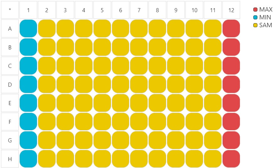
Six serial dilution plates were used. Minimum and maximum controls were placed in columns 1 and 12, respectively.

Raw data was generated by an AnalystGT Reader from Molecular Devices.

Files to use:

• 02-Dose_Response_Assay_p96_Raw_Data
• 02-Sample_Mapping_Dose_Response_Assay_p96

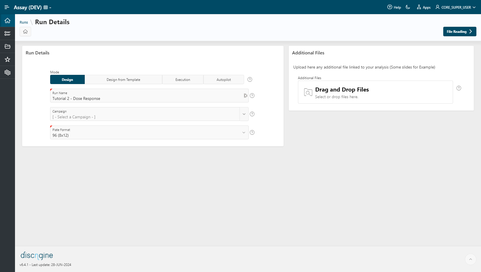
Run Creation

• To create a new run, click the New Run button.
• Select Mode as Design Mode.
• Enter a Run Name.
• Specify the plate format to use: 96 (8x12).
• Go to the File Reading step.

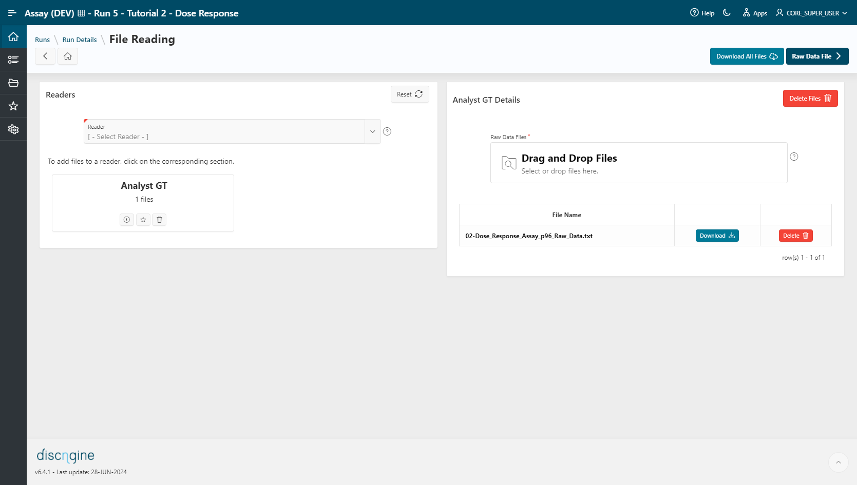
File Reading

• Select Analyst GT (TAB) as a reader.
• Select the file 02-Dose_Response_Assay_p96_Raw_Data in the upload section. The file is automatically uploaded upon selection and listed in the table below.
• Go to the Raw Data File step.

Raw Data File

• The Number of Measurements per Plate (1) and the READOUT Alias (READOUT1) are already set.
• Go to the Plate Mapping step.

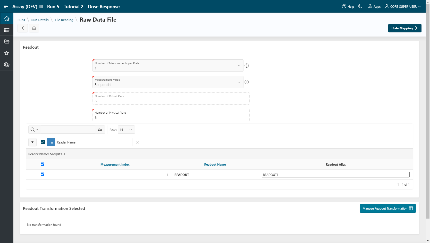
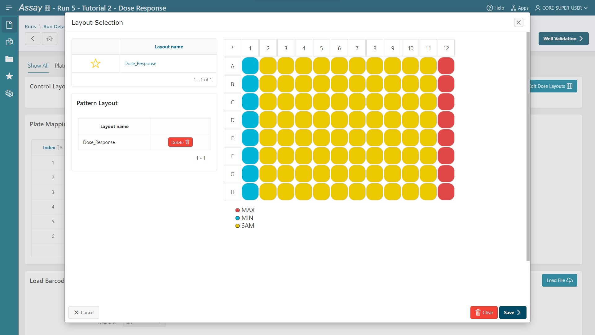
Plate Mapping

• Click Edit Control Layouts.
• Select the Control Layout named Dose_Response (Minimum control in column 1 and maximum control in column 12).
• Click Save.

Info

Barcode information is not needed in this tutorial. This section allows users to set plate barcodes using a file with two columns (Plate_Index / Barcode).

• All your plates have the Dose_Response layout.

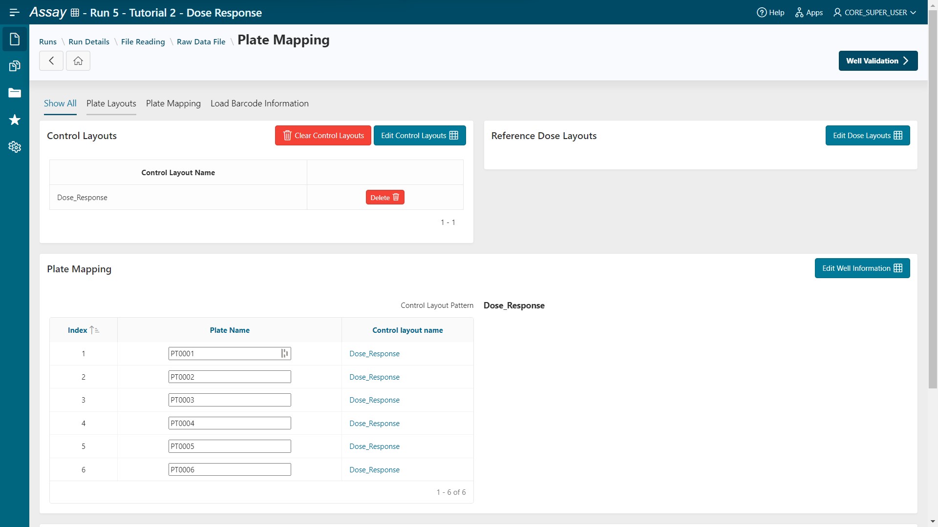
• Go to the Well Validation step.

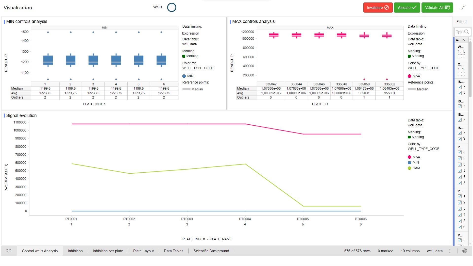
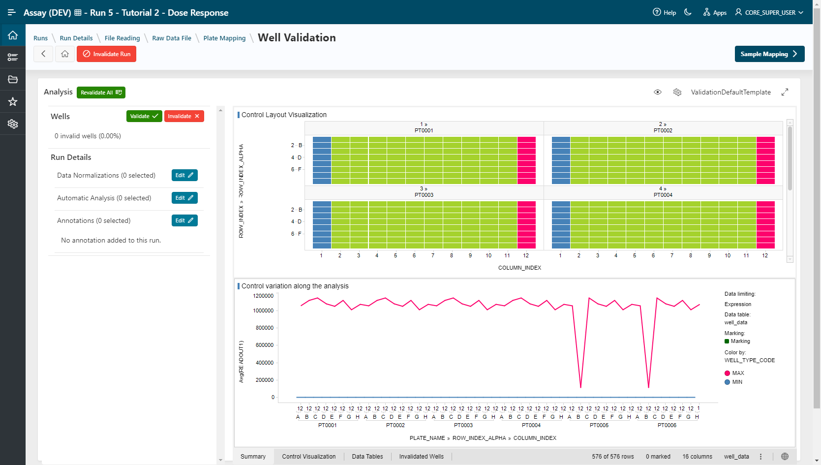
Well Validation

Select your visualization tool:

Info

If you are using Spotfire Analyst Client, or if only one visualization tool is installed in your environment, this step will be skipped.

• TIBCO Spotfire Webplayer (Template: ValidationDefaultTemplate)

• Pipeline Pilot (Template: Well Validation)

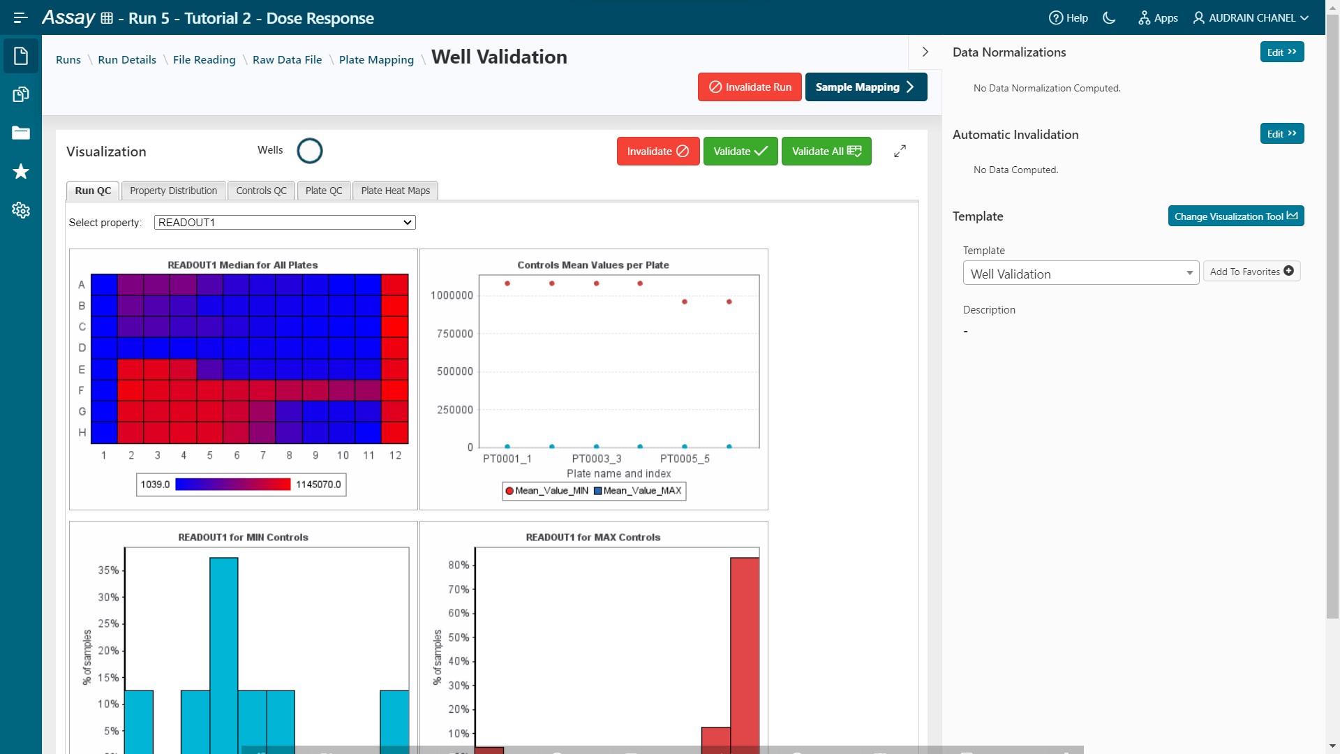
Results are loaded.

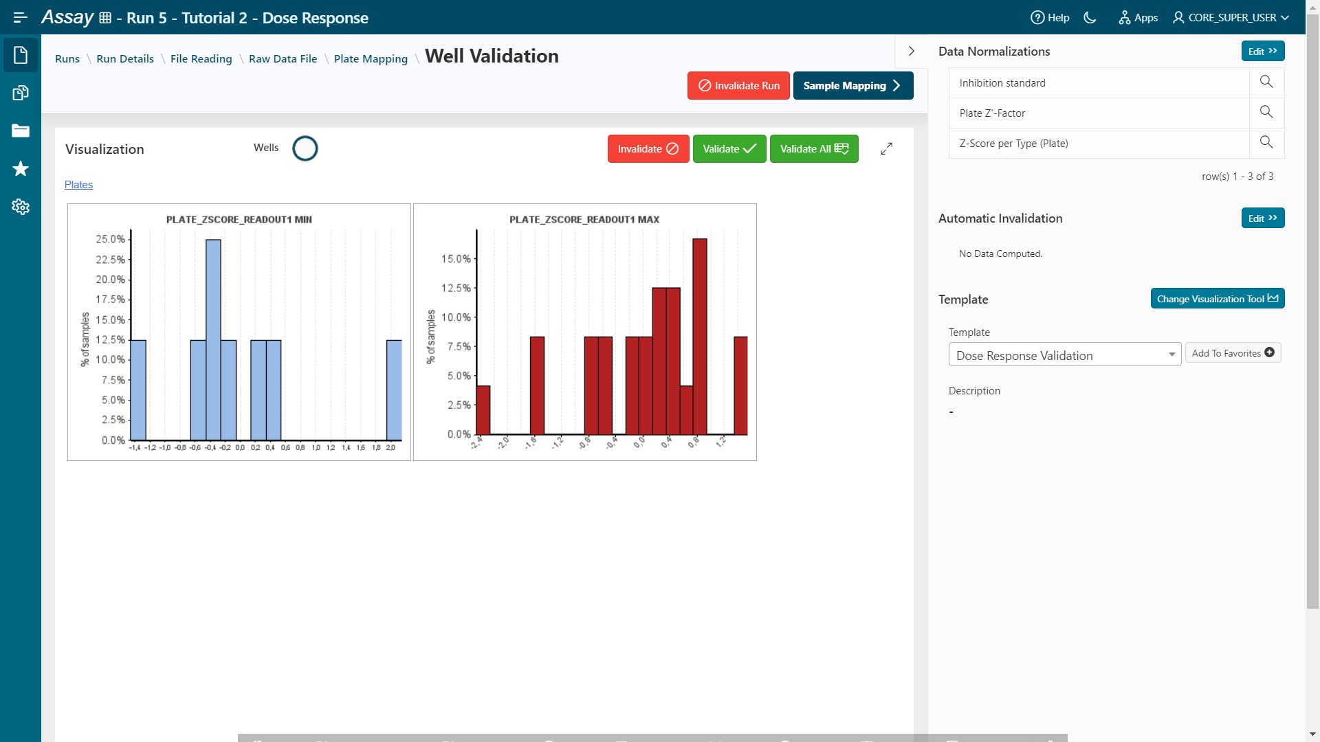
Add Data Normalizations:

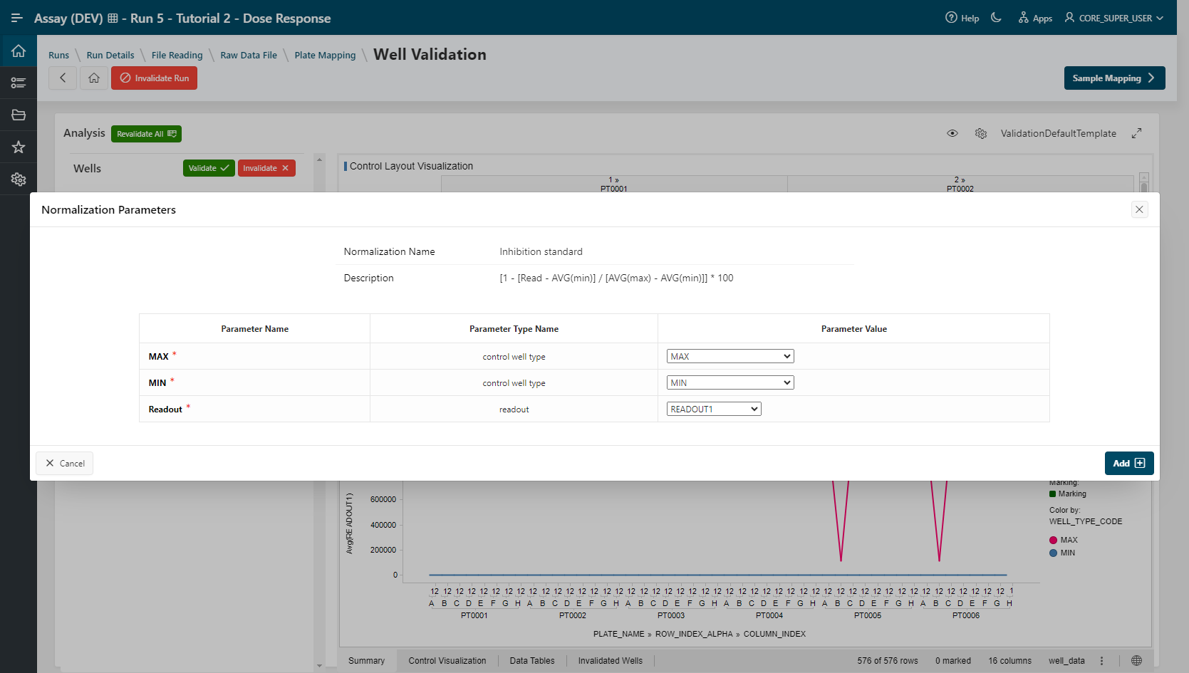
• In the left panel, next to the Data Normalization summary, click Edit to open the Data Normalizations modal.
• Look for the Inhibition Standard procedure and click Add:
  • Value READOUT1, MIN, and MAX are selected.
  • Click Add.

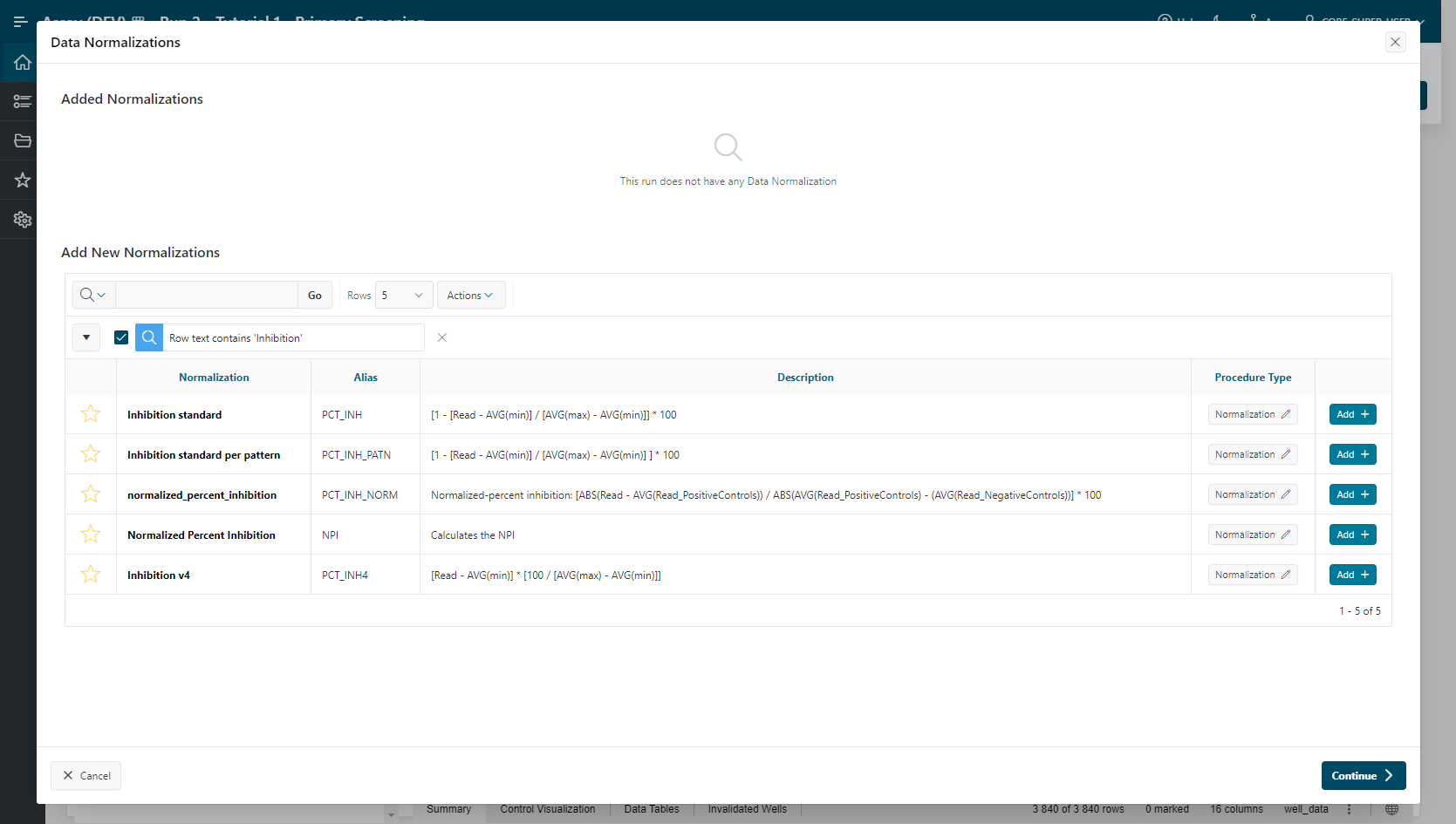
The Inhibition Standard normalization is listed in the Data Normalization Summary section.

• Repeat this action for Plate Z'-factor normalization:
  • Values READOUT1, MIN, and MAX are selected.
  • Click Add.

The Plate Z-factor normalization is listed in the Data Normalization Summary section.

• Repeat this action for Z-Score per Type (Plate) normalization.
  • Value READOUT1 is selected.
  • Click Add.

The Z-Score per Type (Plate) normalization is listed in the Data Normalization Summary section.

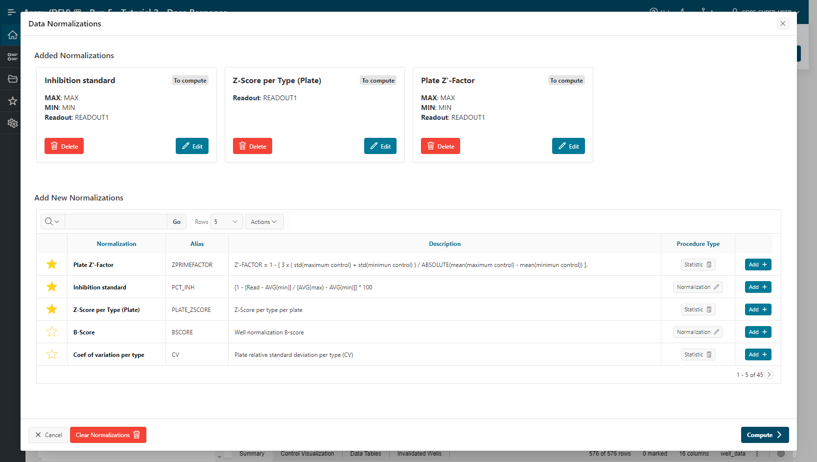
• Click on Compute. You are automatically redirected to the Well Validation page.

All normalizations are processed. Select another visualization template by clicking on the gears button above the current visualization.

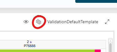
• Apply the Dose_Response_Template (Spotfire)

• Apply the Dose Response Template (Pipeline Pilot)

• Or create a new one and save it (see developer guide to register a new Pipeline Pilot Protocol in Assay).

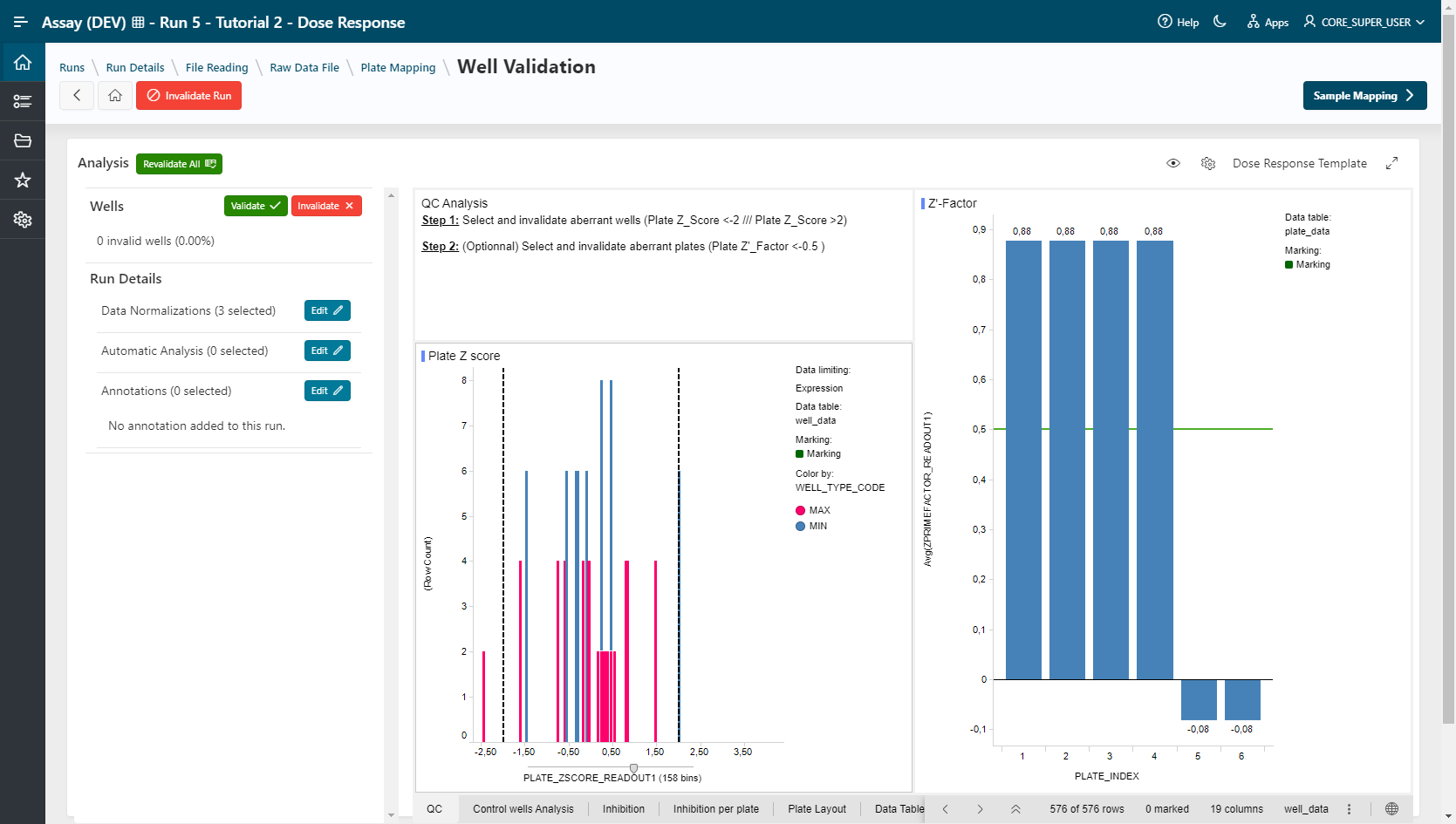
For QC Validation, select aberrant wells in the visualization and click on the button. Multiple selection is allowed by holding the Ctrl key.

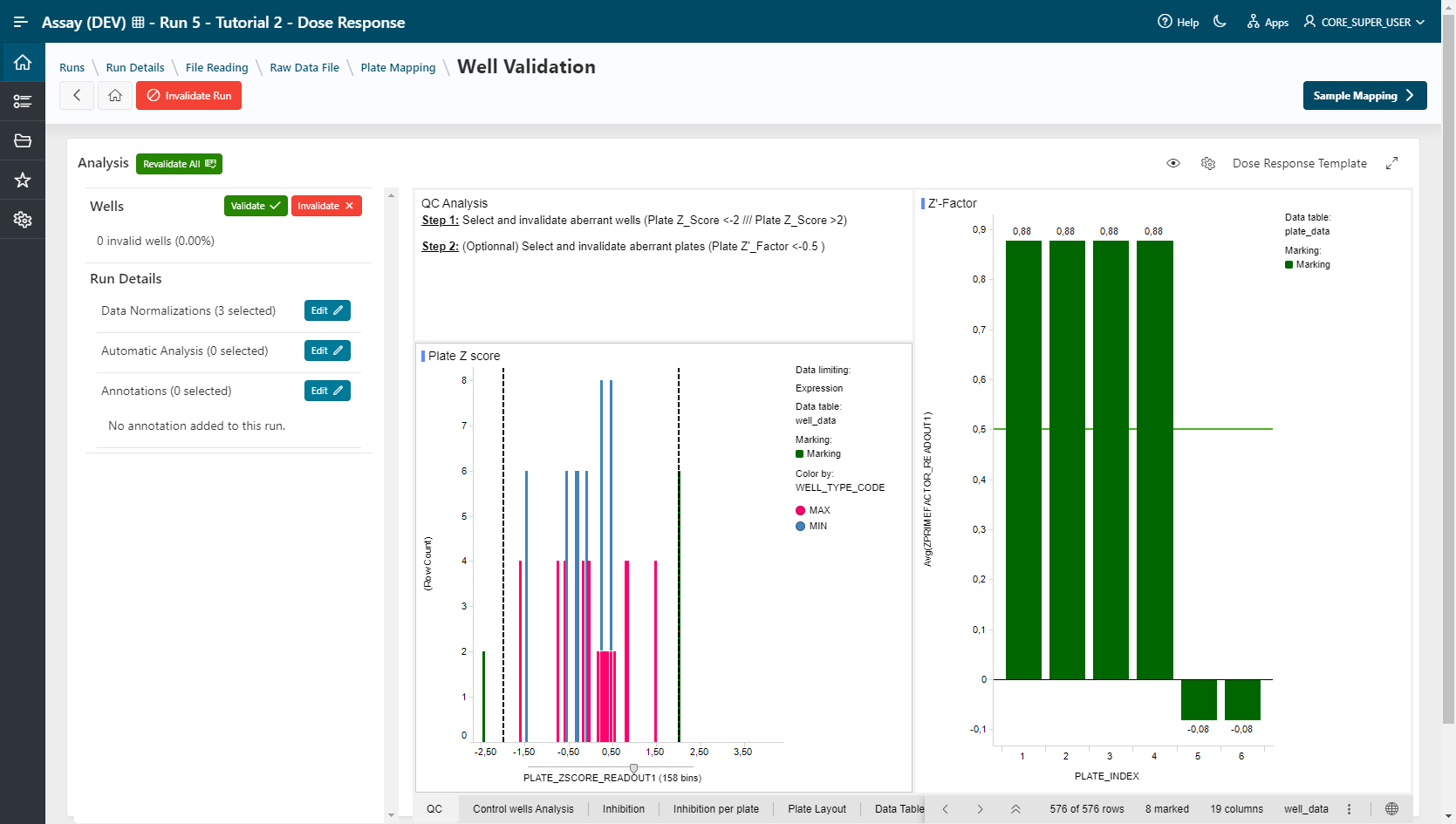
After each invalidation, the normalizations will be relaunched in order to recalculate based on your selection.

Example

Plate_ZSCORE_READOUT1 < -2 or Plate_ZSCORE_READOUT1 > 2. (8 wells are invalidated) and all normalizations are recomputed.

Tip

The space occupied by the visualization can be optimized to your liking by clicking on the icon and the icon

• Go to the Sample Mapping step

Sample Mapping

• Click on Edit Sample Information button.
• Select filling mode File and tick Sample and Dose for content.
• Load the file 02-Sample_Mapping_Dose_Response_Assay_p96.
• Click on Apply button. Samples and doses are filled in.

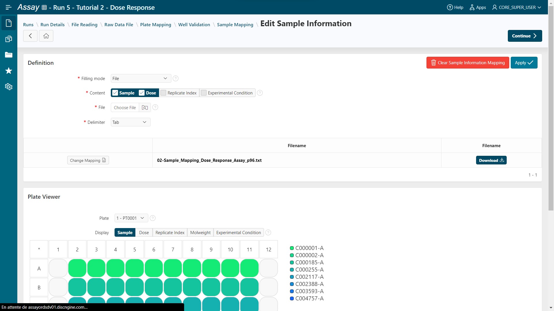
• Click on Continue button.

Samples and doses are mapped for all plates.

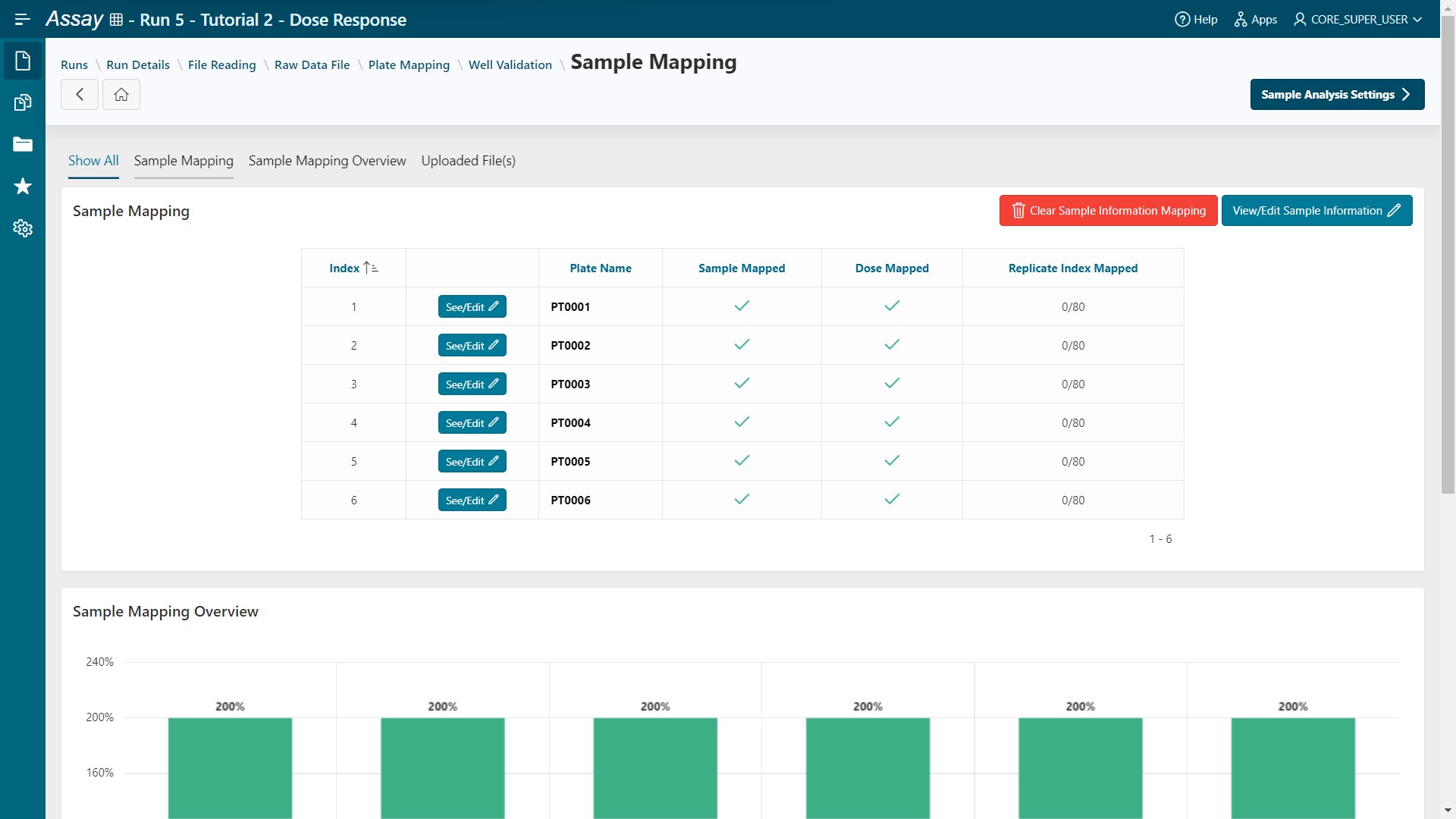
• Click on Sample Analysis Settings button.

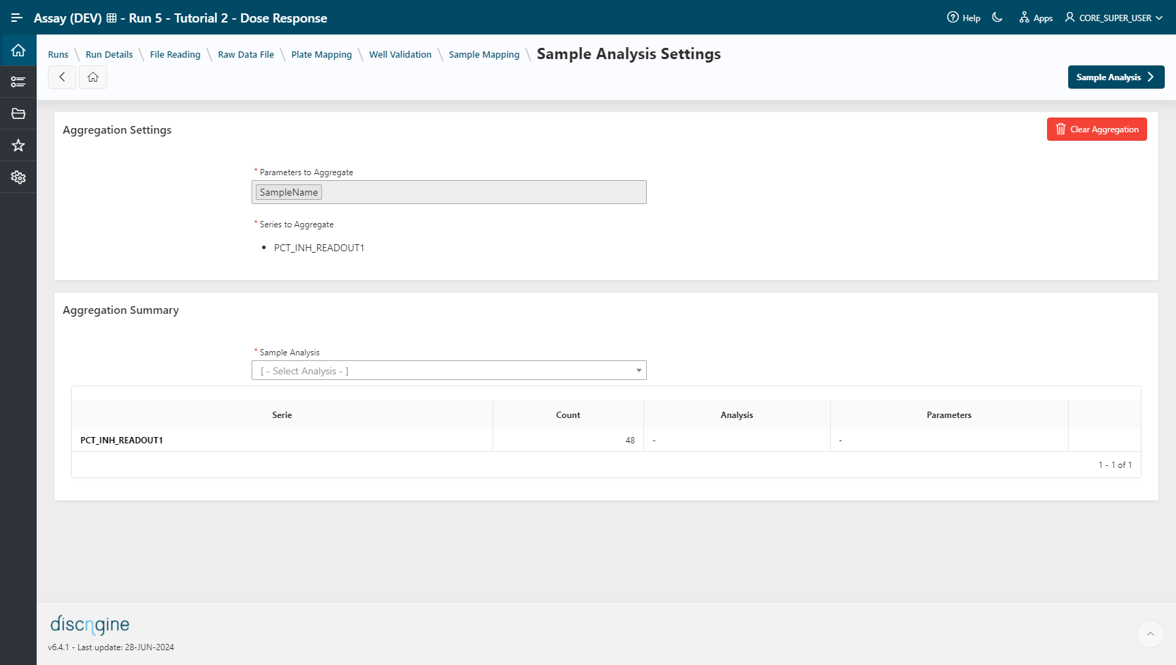
Sample Analysis Settings

• Select the parameter to aggregate: SampleName.
• Select the Series: PCT_INH_READOUT1.
• Click on Create Analysis Groups button: 48 groups are created.

• Select the analysis Dose Response Fitting, then click on the Add Sample Analysis button.
• Leave the parameters empty, click on Save to apply the method to all series.

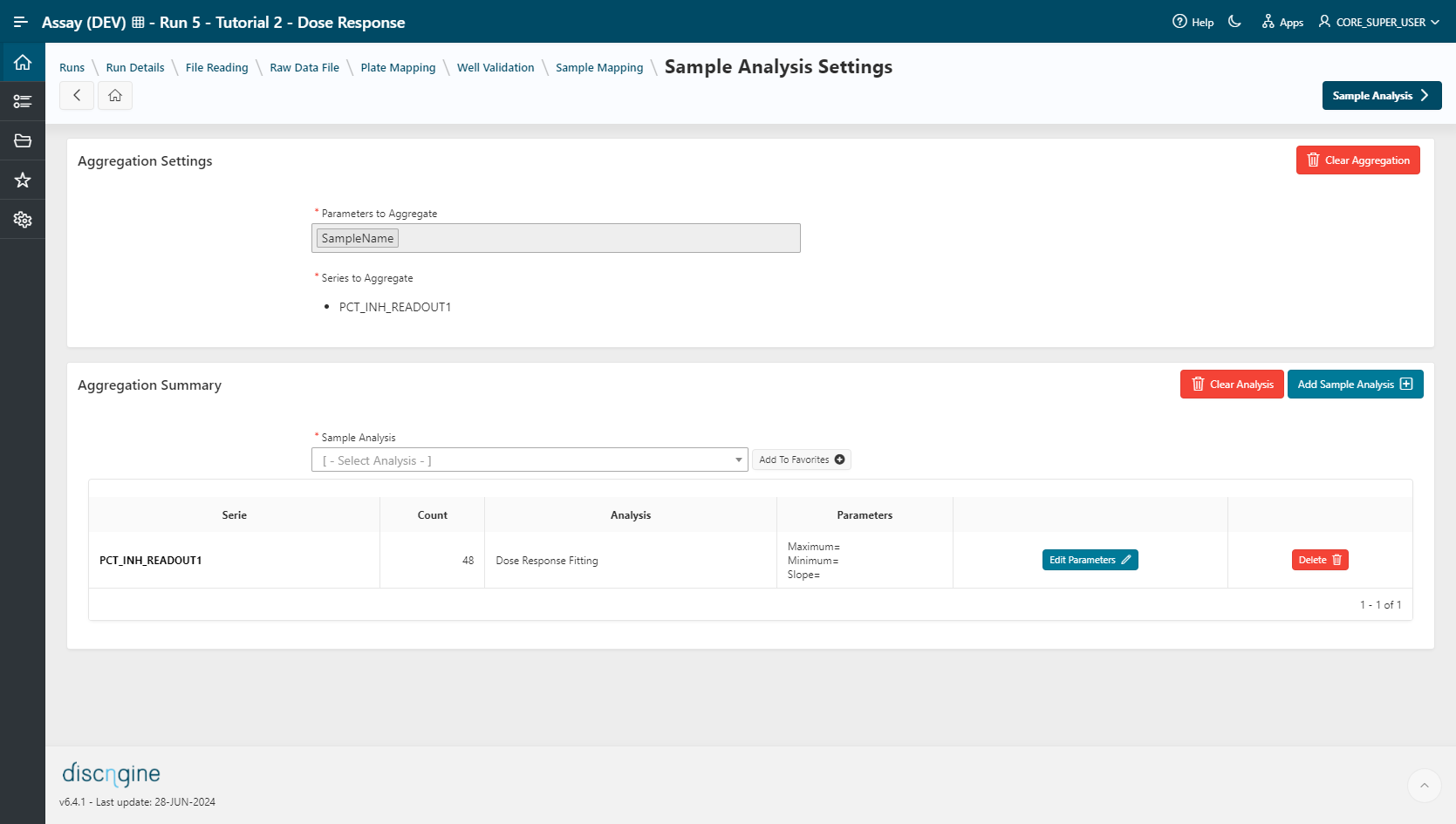
• Go to the Sample Analysis step.

Sample Analysis

Select your Visualization Tool:

• TIBCO Spotfire Webplayer
• Pipeline Pilot

Info

This step is only available if 2 visualization tools are installed. Otherwise, this step will be skipped.

• Apply an existing template
• Dose Response Fitting (Spotfire Template):

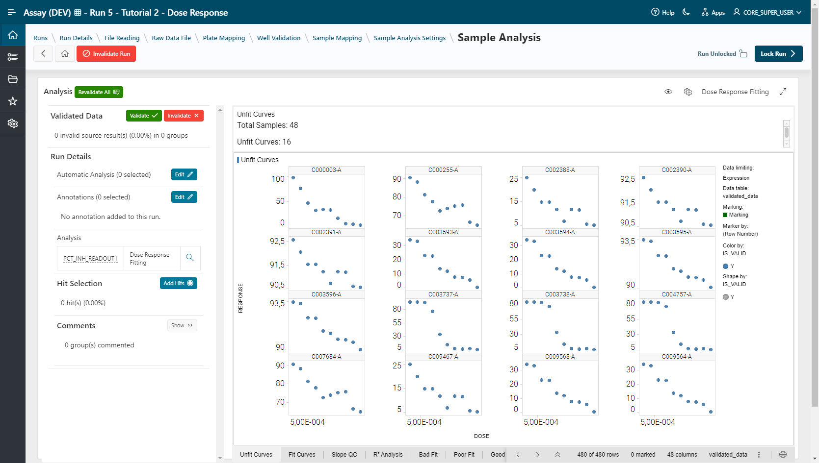
For Hit Selection, select points (hits) in the visualization and add them to a list by clicking on the Add Hits button. This selection can be exported in CSV format (export button) or used to create a list that can be used in the Sample application.

• Lock your Analysis using the Lock Run button.
• Go to Publisher step.

Publisher Selection & Workflow Template Creation

• Select a target publisher (depending on what is installed – None, Warehouse or BIOVIA Project Data). For more information on publishing data see the Publisher guide.

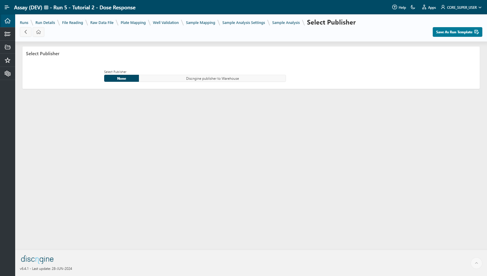
• Save your analysis by clicking on Save As Run Template. The template will be used later in the execution mode.

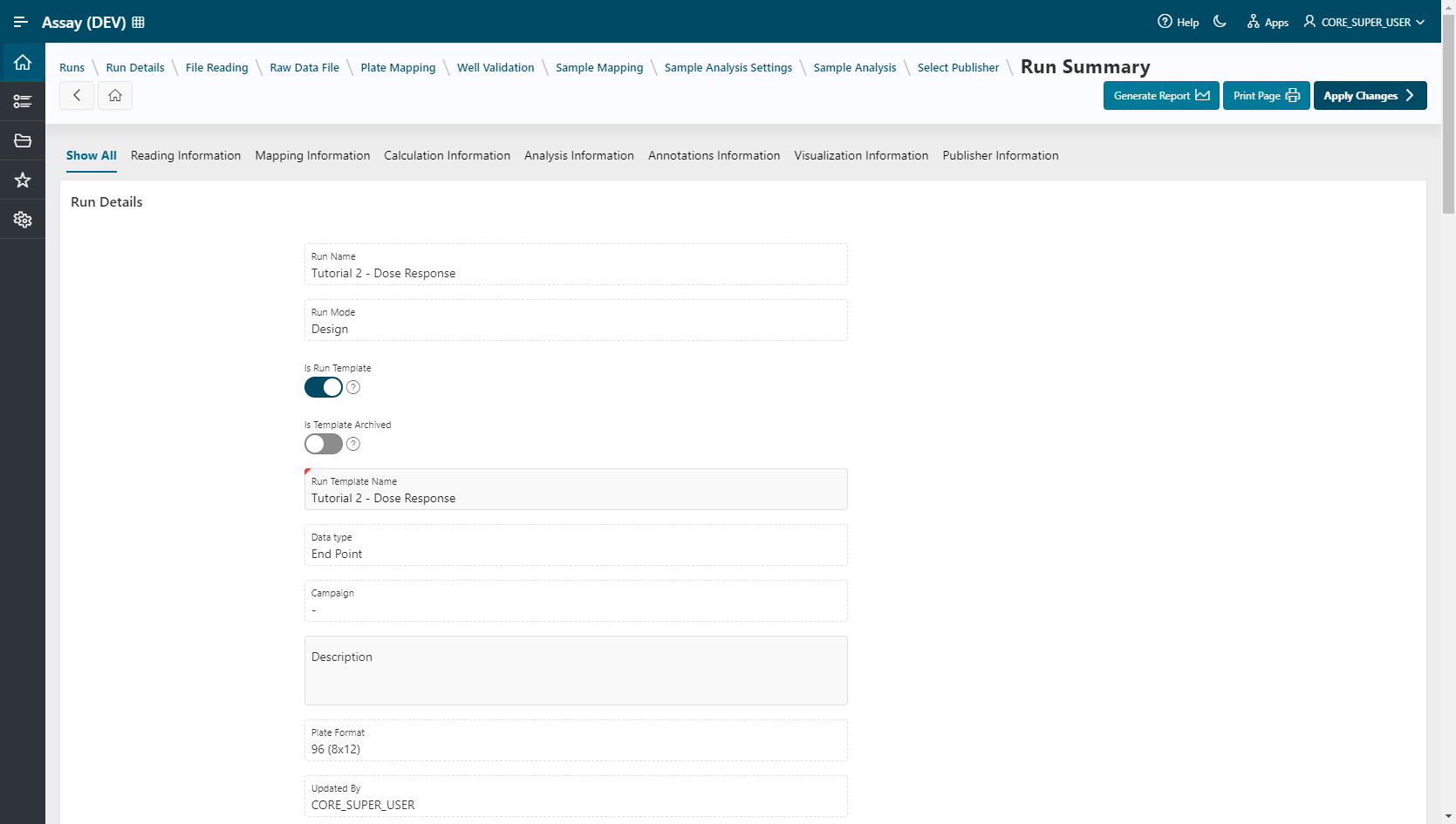
• Give a name and description to the run template.
• Click on Apply Changes to save your modifications.

Info

Once the run template is saved, the screeners can use it in Execution Mode, following this tutorial