ELISA assay

Introduction¶

First described by Eva Engvall and Peter Perlmann in 1971, the enzyme-linked immunosorbent assay (ELISA) is a commonly used analytical biochemistry assay. The assay uses a solid-phase type of enzyme immunoassay (EIA) to detect the presence of a ligand (commonly a protein) in a liquid sample using antibodies directed against the protein to be measured. The ELISA test is the first screening test commonly employed for HIV. It was approved for use on March 2, 1985.

Scientific Background¶

Although HIV antibody tests are the most appropriate for identifying infection, alternate technologies can contribute to an accurate diagnosis, assist in monitoring the response to therapy, and can be used to effectively predict disease outcomes. Viral isolation through viral culture, nucleic acid tests to detect viral RNA, and tests to detect p24 antigen can be used to demonstrate virus or viral components in blood, thereby verifying infection. These methods are highly specific, and a positive result confirms infection. However, each has limitations and their use must be tailored to proper testing situations. Tests for viral nucleic acid have recently been introduced, but require sophisticated technology and dedicated, well-trained personnel.

The HIV antigen test is currently used for screening blood for transfusion and is appropriate for use in several other testing situations. It offers the advantages of simplicity and cost-effectiveness for verifying infection but is less than perfect.

The p24 antigen assay measures the viral capsid (core) p24 protein in blood that is detectable earlier than HIV antibody during acute infection. It occurs early after infection due to the initial burst of virus replication and is associated with high levels of viremia during which the individual is highly infectious. However, when antibodies to HIV become detectable, p24 antigen is often no longer demonstrable, most likely due to antigen-antibody complexing in the blood. When detected, p24 antigen is highly specific for infection.

The goal of this study is to identify compounds that can inhibit HIV replication in latently infected cells.

Materials and Methods¶

A microplate is prepared containing a blank, positive and negative controls, the standards, and the samples.

Controls¶

For confidence in ELISA results, it is necessary to have three experimental controls for comparison: a positive control, negative control, and a standard control. Both the positive and standard controls are known to contain the protein or peptide of interest.

The positive control is to confirm that the procedure is performing as intended.

The negative control is known to not contain the biomolecule of interest, and adds validity to any positive results.

The standard control is necessary for quantification of the experimental results. It contains a known quantity of the target molecule and therefore gives the information necessary to make a standard curve.

Standards¶

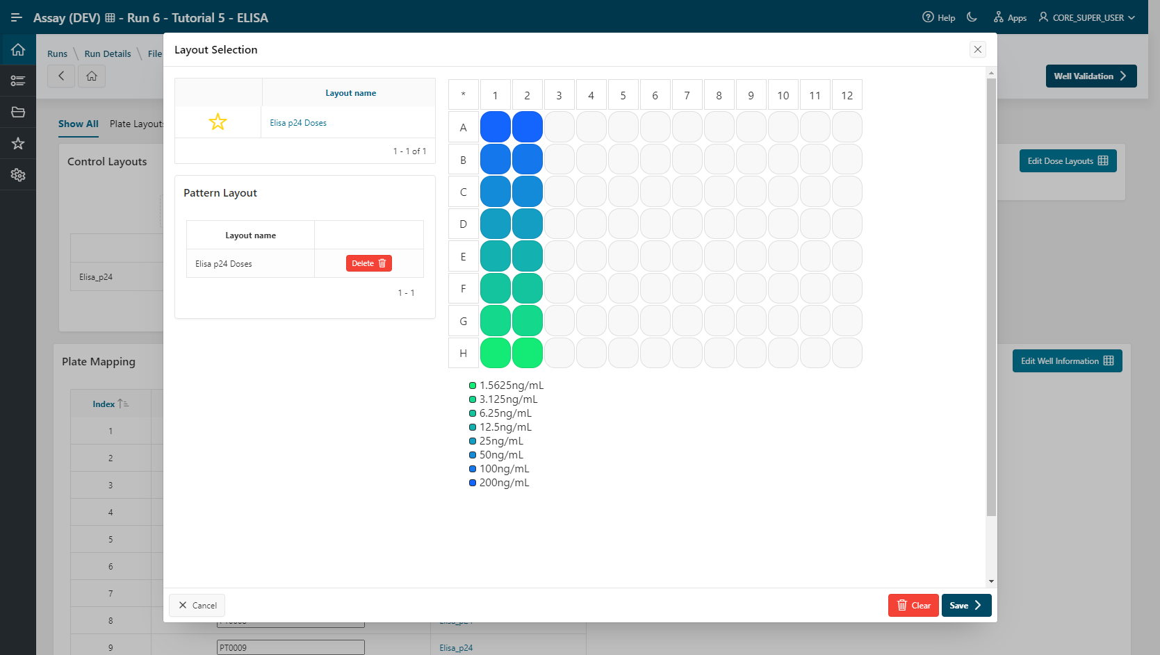
To determine the levels of p24 antigen in latently infected cells, an HIV-1 antigen standard is diluted to prepare a series of eight standards of varying concentrations. Concentrations vary between 0.0 and 200 ng/mL.

Samples¶

For this study, we use two cloned cells chronically infected with HIV-1: U1 and OM10.1. To prepare the samples, the cells are incubated with different compounds to test.

Principle¶

The optical densities at 490 nm and 650 nm are measured for the microplate and the ratio of both measurements is calculated. These values are then corrected with the mean of the blank wells' optical densities.

A standard curve is generated using a linear graph and plots the concentration of the HIV-p24 antigen standard (ng/mL) on the X-axis versus the mean optical densities for each standard on the Y-axis. Each standard is added in duplicate wells.

Then the optical density values of the unknown specimens (samples) are interpolated in the standard curve to determine their concentration using linear regression.

If the value of the unknown sample is higher than the value of the highest standard, the sample must be diluted and the entire neutralization procedure is repeated.

Third-Party Software¶

This tutorial was developed using TIBCO Spotfire 11.4. Visualization templates may need adjustments if using older versions of that software.

Dataset¶

Prerequisite: Control Layout Elisa_p24 and Dose Layout Elisa p24 Doses must exist.

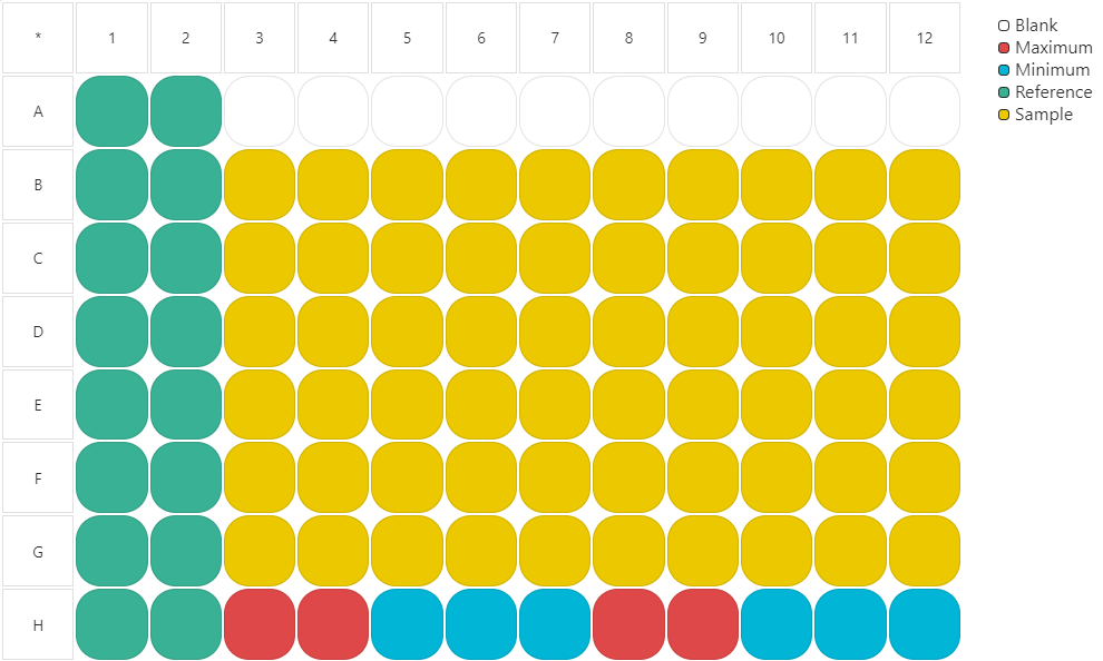
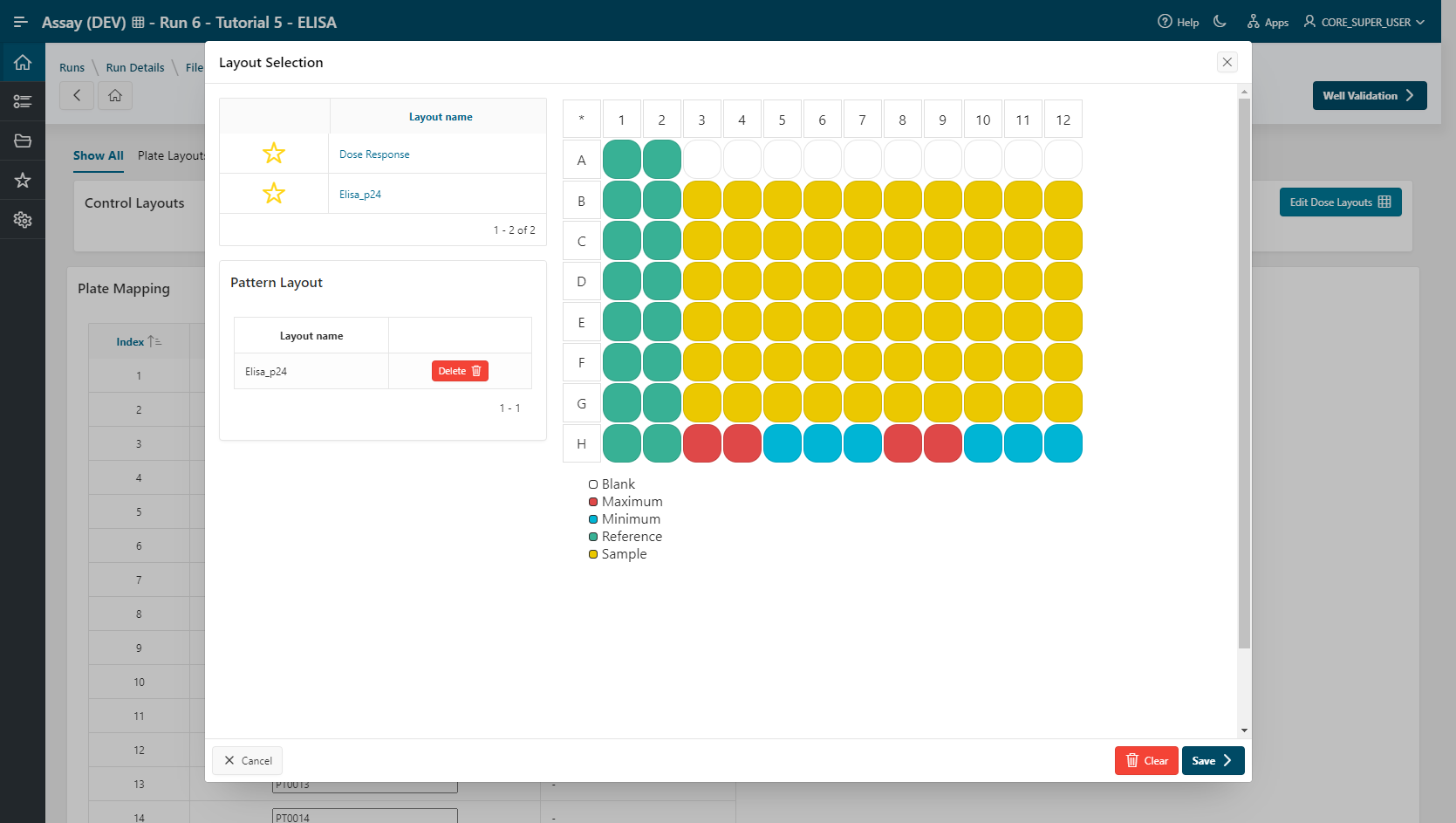
Fifty plates are used. References (standards) are placed in duplicate in columns 1 and 2. Blanks are placed in wells A3-A12. Samples are placed in wells B3-G12. Positive and negative controls are placed in wells H3-H12.

Control Layout for ELISA — Plate Layout for ELISA

Files to use:

Run Creation¶

To create a new run, click New Run.
Select Mode as Design Mode.
Enter a Run Name.
Specify the plate format to use: 96 (8x12).
Go to the File Reading step.

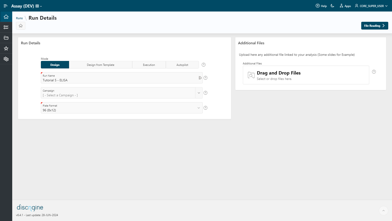
Run Template is mandatory only in Execution Mode. This option in Design Mode can be used to create a new analysis based on an existing workflow template.

File Reading¶

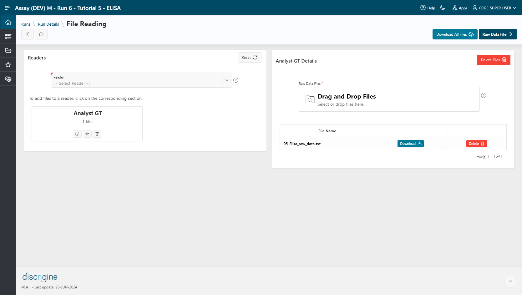
Select Analyst GT (TAB) as a reader.
Click Reader Information to view information about the selected reader.
Select the file 05-Elisa_Raw_Data in the upload section. The file is automatically uploaded upon selection and listed in the table below.
Go to the Raw Data File step.

Raw Data File¶

Modify the parameters of the Reading Mode:

Number of Measurements per Plate: 2.
Measurement Mode: Sequential.
The number of virtual plates is fixed to 100.
The number of physical plates is fixed to 50.
Rename READOUT1 to READOUT490, which represents the optical density measured at 490 nm.
Rename READOUT2 to READOUT650, which represents the optical density measured at 650 nm.

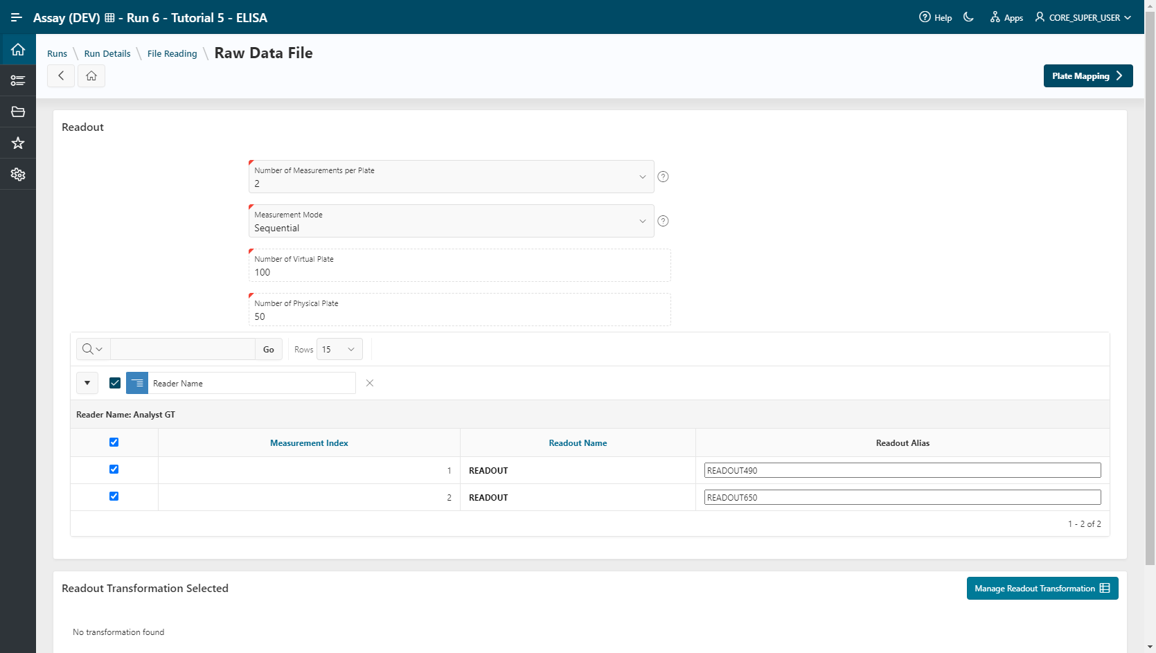
Raw Data File step : Adjust number of measurement and mode

Click on Continue to go to the Plate Mapping step.

Plate Mapping¶

Click on Edit Control Layouts.
Select the default control layout named Elisa p24 (References, samples, blanks and Min/Max are displayed as explained in Dataset).
Click on Save.

Click on Edit Dose layouts.
Select the Dose Layout named Elisa p24 Doses (Doses from 200 to 1.5625 in columns 1 and 2).
Click on Save.

Info

Editing well information is possible (e.g., add experimental conditions).

Go to the Well Validation step.

Well Validation¶

Select your Visualization Tool: TIBCO Spotfire Webplayer

Info

If you are using Spotfire Analyst Client, or if only one visualization tool is installed on your environment, this step will be skipped.

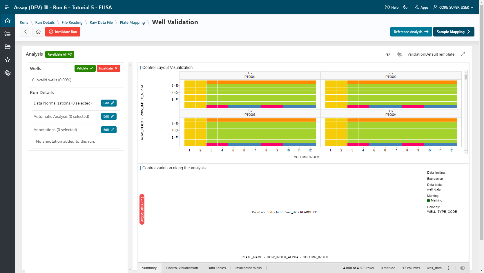
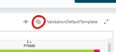
Select the template ValidationDefaultTemplate and click Next.

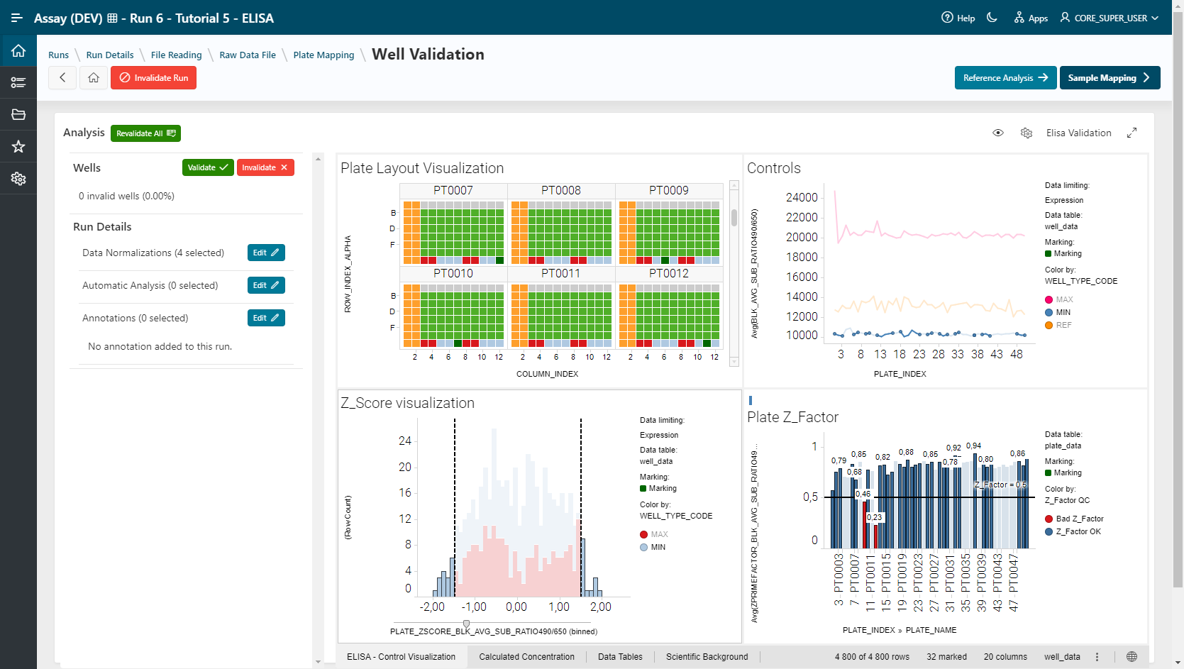
Results are loaded:

The first visualization corresponds to the representation of the layout for each plate. The second visualization corresponds to the optical density measurement of the controls and the blank.

To validate the standard curve that will be generated with a Linear Regression normalization, first we will correct the optical densities obtained by the mean of the blank wells by a subtraction calculation. Then we will calculate the Z' factor and the Plate Z-score to invalidate the abnormal points.

Add Data Normalizations:

In the left panel, next to the "Data Normalization" summary, click Edit to open the Data Normalizations modal.
Look for the "Readout Transformation - Divide" procedure and click on Add
- Set RATIO490/650 as Output name
- Select READOUT490 as Readout 1
- Select READOUT650 as Readout 2
- Click on Add

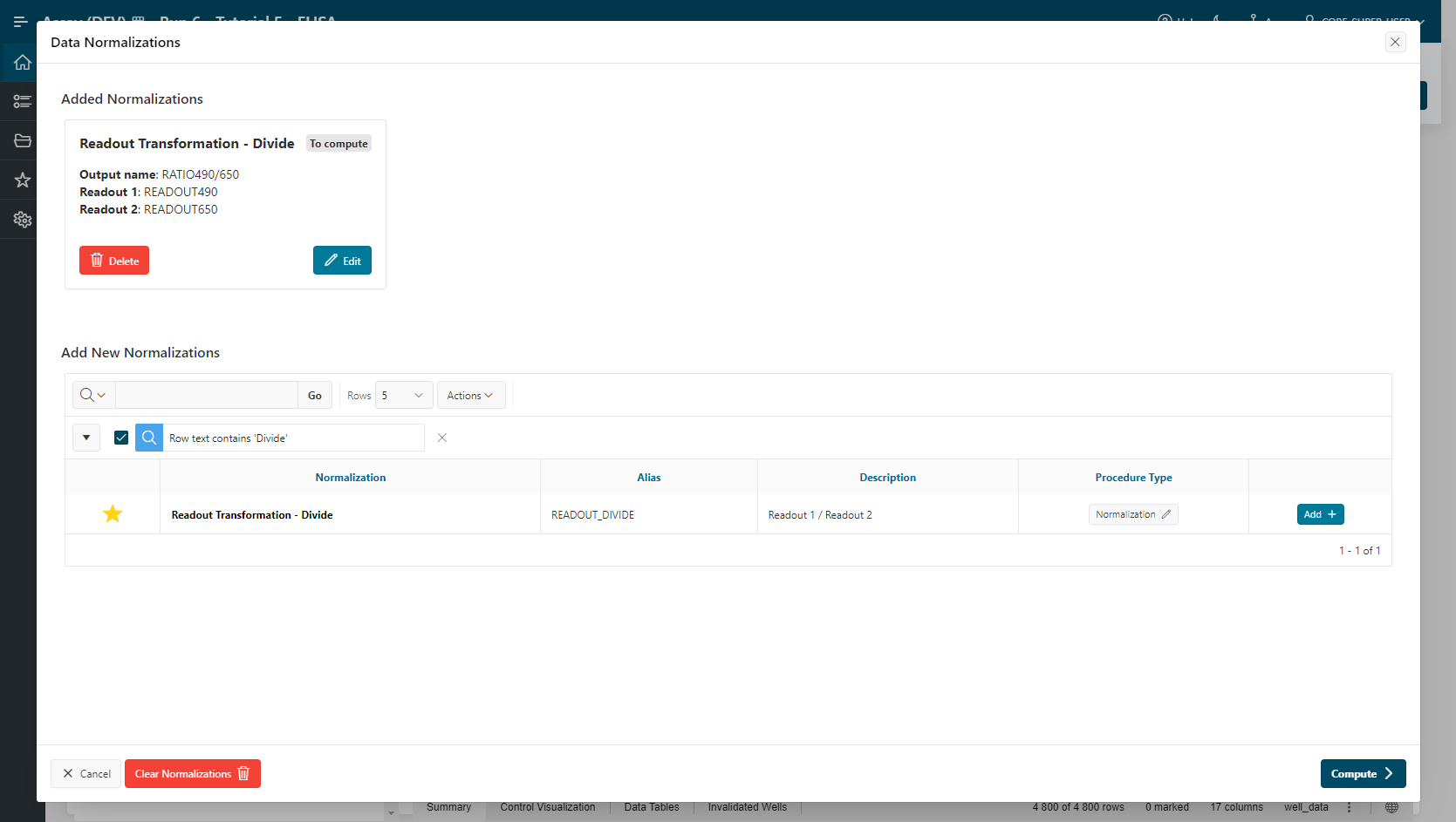
Since the output of this normalization is required for other normalizations to run, we must first compute it. Click on Compute

The normalization is computed and added to the Summary.

Tip

If you wish to remove a normalization that is already computed, you must clear all normalizations with the button Clear Normalizations

Do the same with these other normalizations.

Add the Average Subtraction normalization:
- Select RATIO490/650 as Readout Value
- WELL TYPE Value BLK is selected
- Click Add
- Click Compute (required for other normalizations)
Add the Plate Z'-factor normalization:
- Select BLK_AVG_SUB_RATIO490/650 as Readout value
- Select - CTRL as Minimum Control
- Select + CTRL as Maximum Control
Add the Z-Score per Type (Plate)
- Select BLK_AVG_SUB_RATIO490/650 as Readout Value
- Click Add
- Click Compute

All normalizations are processed.

Select another visualization template by clicking on the gears button above the current visualization.

Well Validation step: Change visualization

Apply the template Elisa Validation

For QC Validation, invalidate points following "Business rules".

Example 1: Plate ZScore interval

Plate_ZSCORE < -1.5 or Plate_ZSCORE > 1.5. Select and invalidate the points out of this scope.

Example 2: Z' factor interval

The Z' factor is an indicator of the statistical data quality for a bioassay.

Being Z' factor between 0 and 1, a Z' factor of 1 is ideal.
A Z' factor between 0.5 and 1.0 is an excellent assay.
A Z' factor between 0 and 0.5 is marginal.
A Z' factor less than 0 means that the signal from the positive and negative controls could overlap, making the assay not very useful for screening purposes.

Select aberrant wells in the visualization and click on the Well Validation step: Invalidation button button. Multiple selection is allowed by holding the Ctrl key.

After each invalidation, the normalizations will be relaunched in order to recalculate based on your selection.

Tip

The space occupied by the visualization can be optimized to your liking by clicking on the full screen icon icon and the icon

QC Validation process-invalidating points

Invalidated points are deleted and the results are recomputed.

In order to finish the QC validation, we still require the normalization Linear Regression. As this calculation requires curve parameters calculated from references, we need to analyze the references.

Click on Reference Analysis →

Now we want to visualize the Reference curve generated from the standards.

Parameters to Aggregate: Reference and PlateIndex.
Series to Aggregate: RATIO490/650.
Click on Create analysis group (50 groups are created).

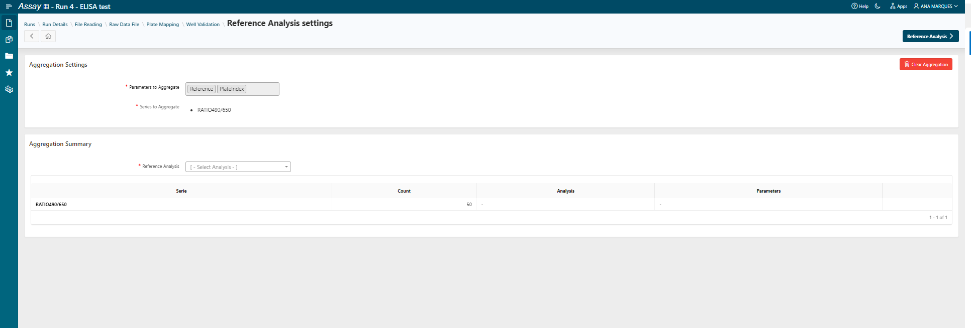
Select Reference analysis Linear Regression Fitting
Click on Add Reference Analysis.
Click on Save in order to set the analysis parameters.

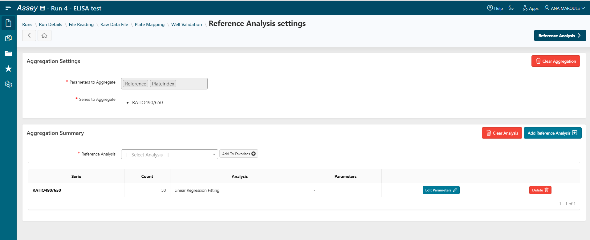
Click on Reference Analysis to apply Linear regression fitting.
All reference analysis is processed.
You are redirected to the Reference Analysis visualization step.
Change the visualization template to Reference Linear Regression.

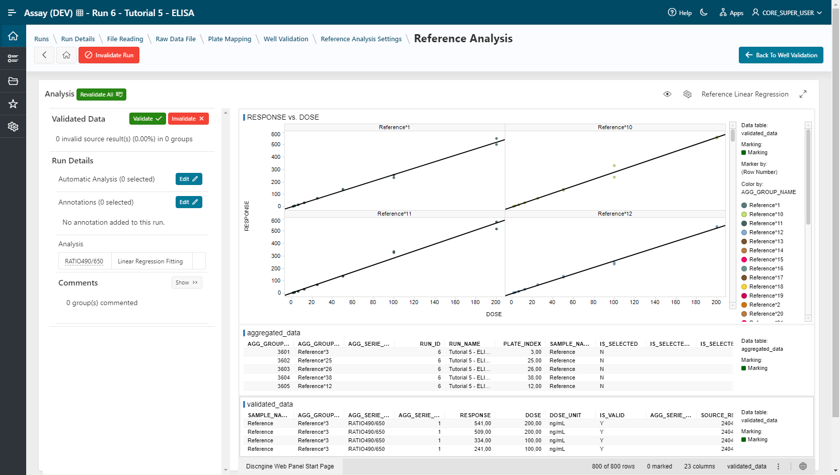
Go Back To Well Validation to finish the QC validation process.
Add the Linear Regression normalization:
- Select BLK_AVG_SUB_RATIO490/650

The Linear Regression normalization is listed in the Data Normalization Summary section.

In the visualization, the calculated concentrations can be displayed in the second tab Calculated Concentration.

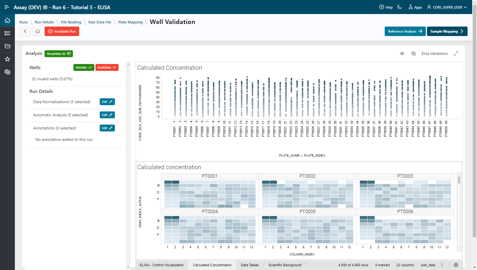
Well validation step: Calculated Concentrations — Calculated Concentrations

When the QC validation process has been completed, we can continue with the next step of the workflow.

Go to the Sample mapping step.

Sample Mapping¶

Select filling mode File and tick Sample, Dose and "Experimental Condition" boxes.
Load the file 05-Elisa_data_mapping+ECD.txt
Click on Manage Experimental Condition in order to create new experimental conditions. Name: CELLS Code: CELLS
Click on Add.
Choose the delimiter Tab.
Click on Apply.

Samples, doses and experimental conditions are filled in:

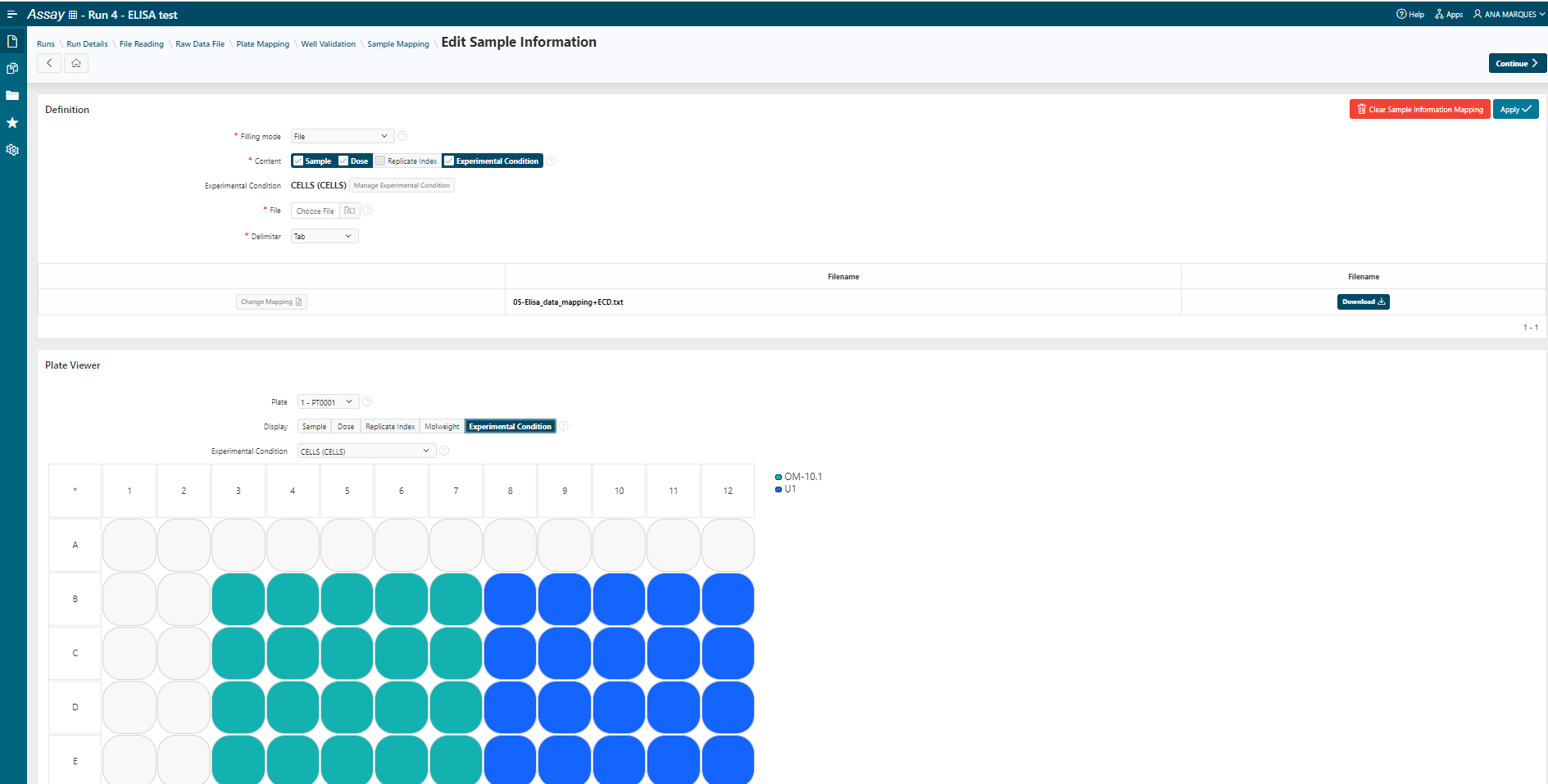
Click on Continue.

Samples, doses and experimental conditions are mapped for all samples. Editing by plate is possible if needed.

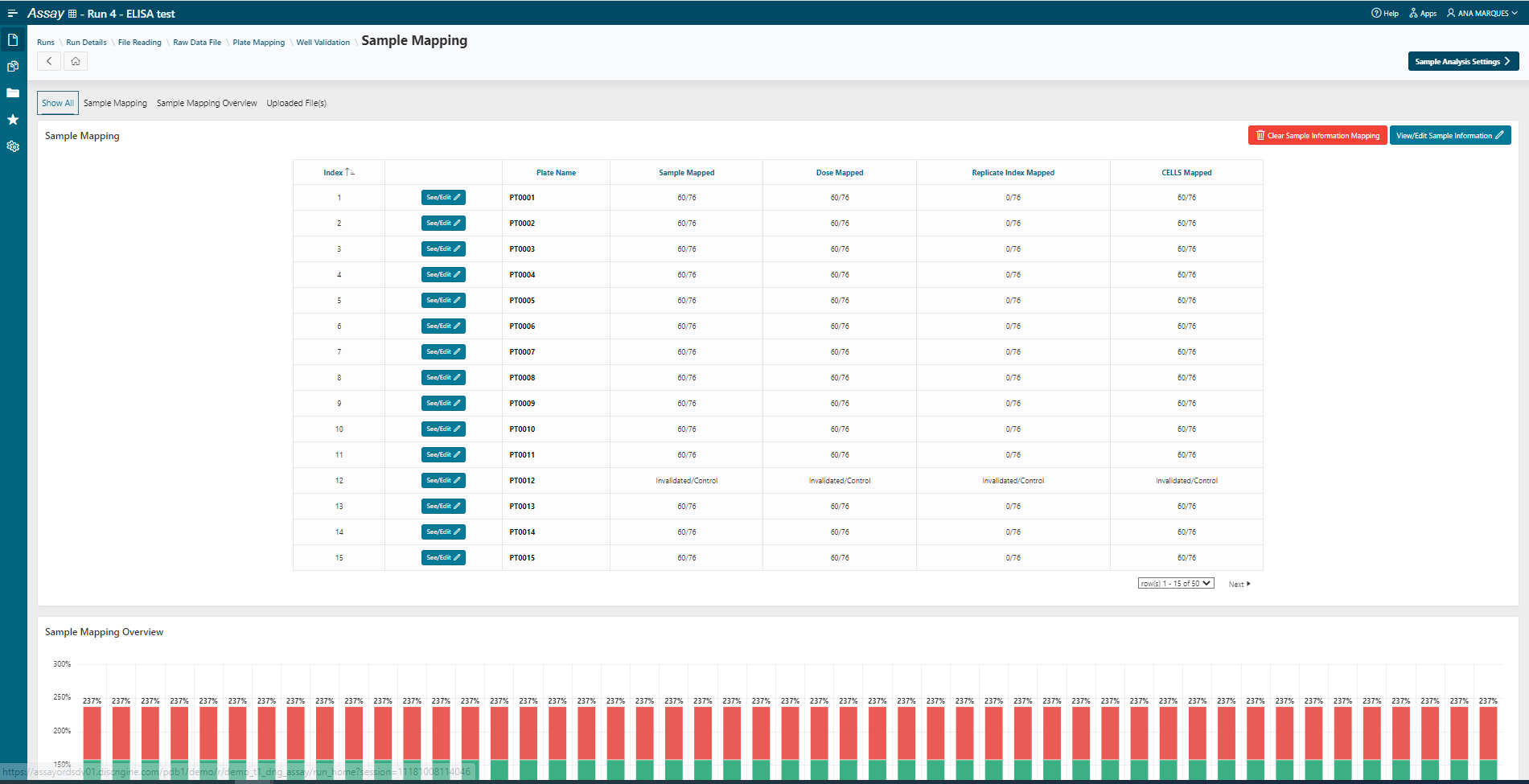
Go to the Sample Analysis Settings step.

Sample Analysis Settings¶

Select the Parameters to Aggregate: SampleName and CELLS.
Select the Series: CONC_BLK_AVG_SUB_RATIO490/650.

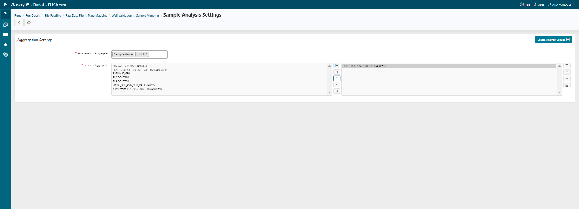
Click on Create Analysis Groups: 1000 groups are created.
Select the Analysis Basic Statistics then click on Add.
Click on Save to apply basic statistics to all series.

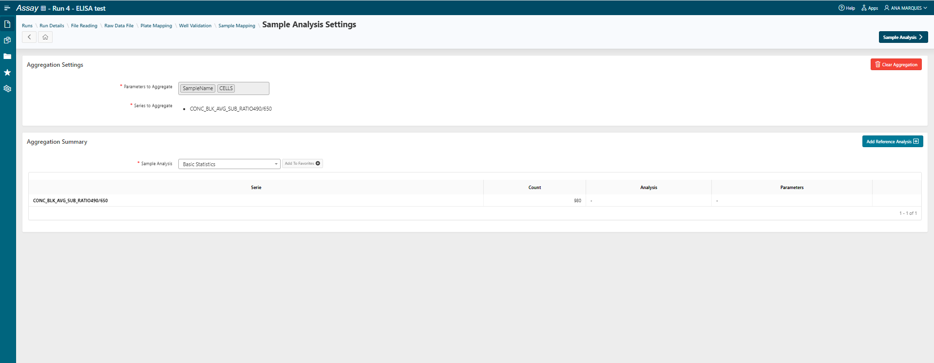
Go to the Sample Analysis step.

Sample Analysis¶

Apply the Elisa Analysis template

The results of the sample analysis are displayed.

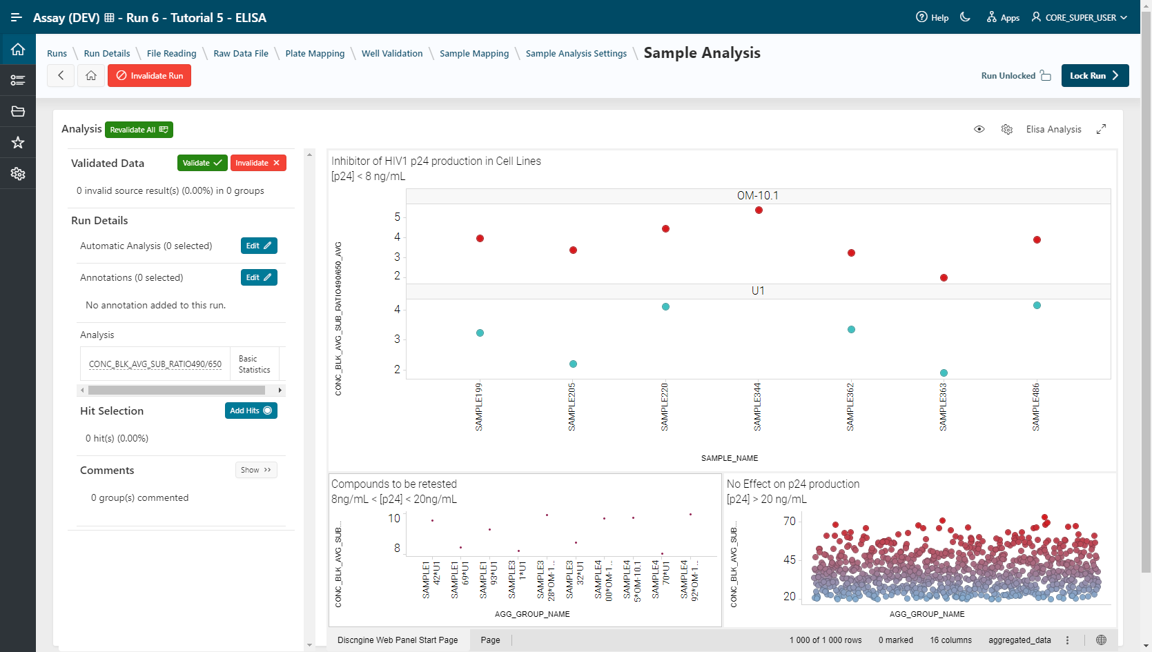
The first visualization shows the samples that have performed a better inhibition of p24 antigen production ([p24]<8 ng/ml) for both U1 and OM10.1 cells, so we can consider them as "Hits".

The second visualization shows the samples that could be retested. The concentration of p24 antigen on cells after the analysis is between 8 and 20 ng/ml.

The third visualization shows the compounds that have no effect on p24 production due to the high concentration of p24 antigen on cells remaining after the analysis (>20 ng/ml).

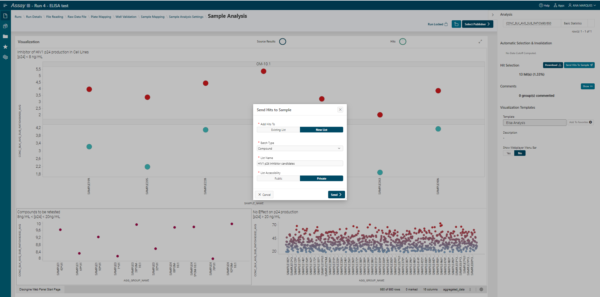
Select the points (hits) in the visualization and click on to add them to a list.

This list can be downloaded and shared or sent to the Sample application for further analysis of these samples.

If the assay is completed, it can be locked and published.

If the assay is locked, you can review the different steps of the workflow but modifications are not allowed. The assay must be locked to be published.

Lock your Analysis.
Go to the Publisher step.

Publisher Selection & Workflow Template Creation¶

You can select a target publisher. Discngine Publisher to Warehouse is the publisher by default but others may be installed. For more information on publishing data see the Publisher guide.

Select None
Save your analysis template by clicking on Save As Run Template. The templates are stored in the system and can be used in Execution mode.
Give a name and description to the run template. The entire workflow information of the assay is displayed as a summary.

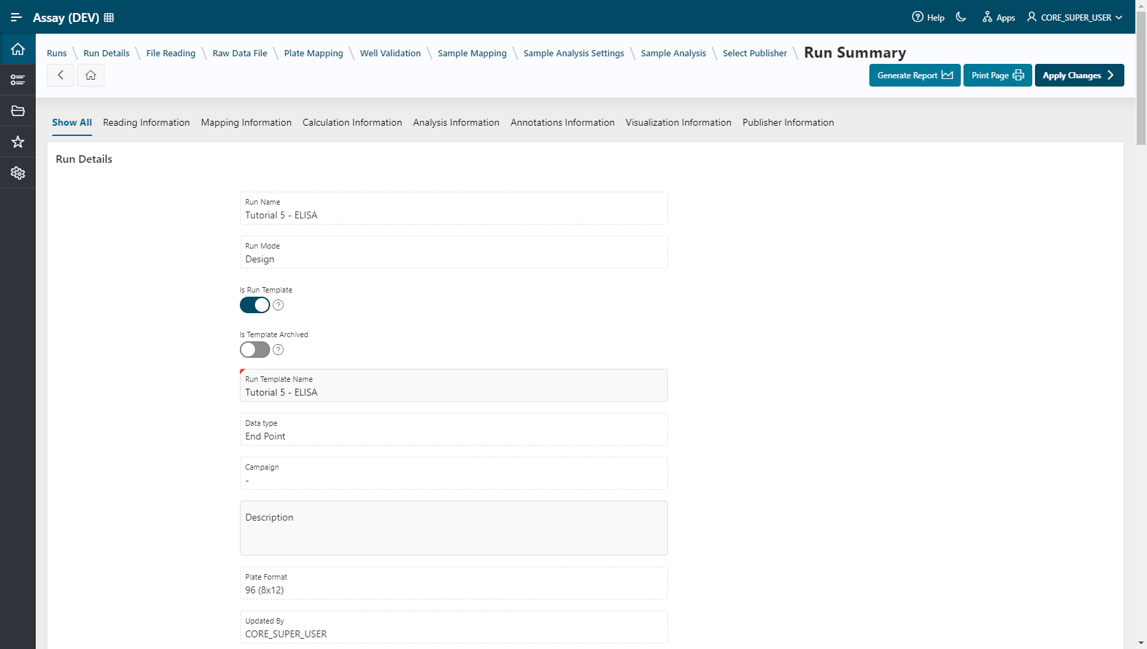
Click on Apply changes and your template is saved.

Info

Once the run template is saved, the screeners can use it in Execution Mode, following this tutorial