Primary Screening

Scientific Background¶

Compound cytotoxicity is an important parameter to measure when developing potential human therapeutics.

Jurkat clone E6.1 was screened against a diverse collection of 3,520 compounds. All compounds were tested once at a 1 μM final concentration.

A luciferase-based cell proliferation/viability assay endpoint kit was used as the readout for this assay. The kit measures the amount of ATP present in the microtiter plate well. If ATP is not present, the catalytic conversion of luciferin into oxyluciferin is not possible, and no luminescence results. Since metabolically active cells produce ATP, the absence of ATP correlates with the presence of non-viable cells.

This campaign was run with doxorubicin, an antibiotic used as an anti-cancer drug, as the positive control. The assay was conducted in 384-well format.

To select a practical number of compounds that exhibited high activity in the primary screen for follow-up assays, a cutoff value of the primary %Inhibition was applied. The cutoff value was calculated as the sum of the average percent inhibition of all compounds tested and three times their standard deviation (= HITS).

Primary Screening Analysis with ASSAY

Third-Party Software¶

This tutorial was developed using BIOVIA Pipeline Pilot 2021 R2 and TIBCO Spotfire 11.4. Visualization templates may need adjustments if using older versions of this software.

Dataset¶

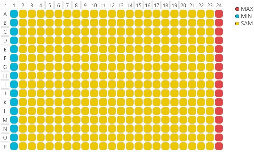
Prerequisite: Control Layout Primary Screening must exist. Ten plates were used, with minimum and maximum controls placed in columns 1 and 24, respectively.

Plate Layout for Primary Screening Analysis

Raw data was generated by an AnalystGT Reader from Molecular Devices. Files to use:

Run Creation¶

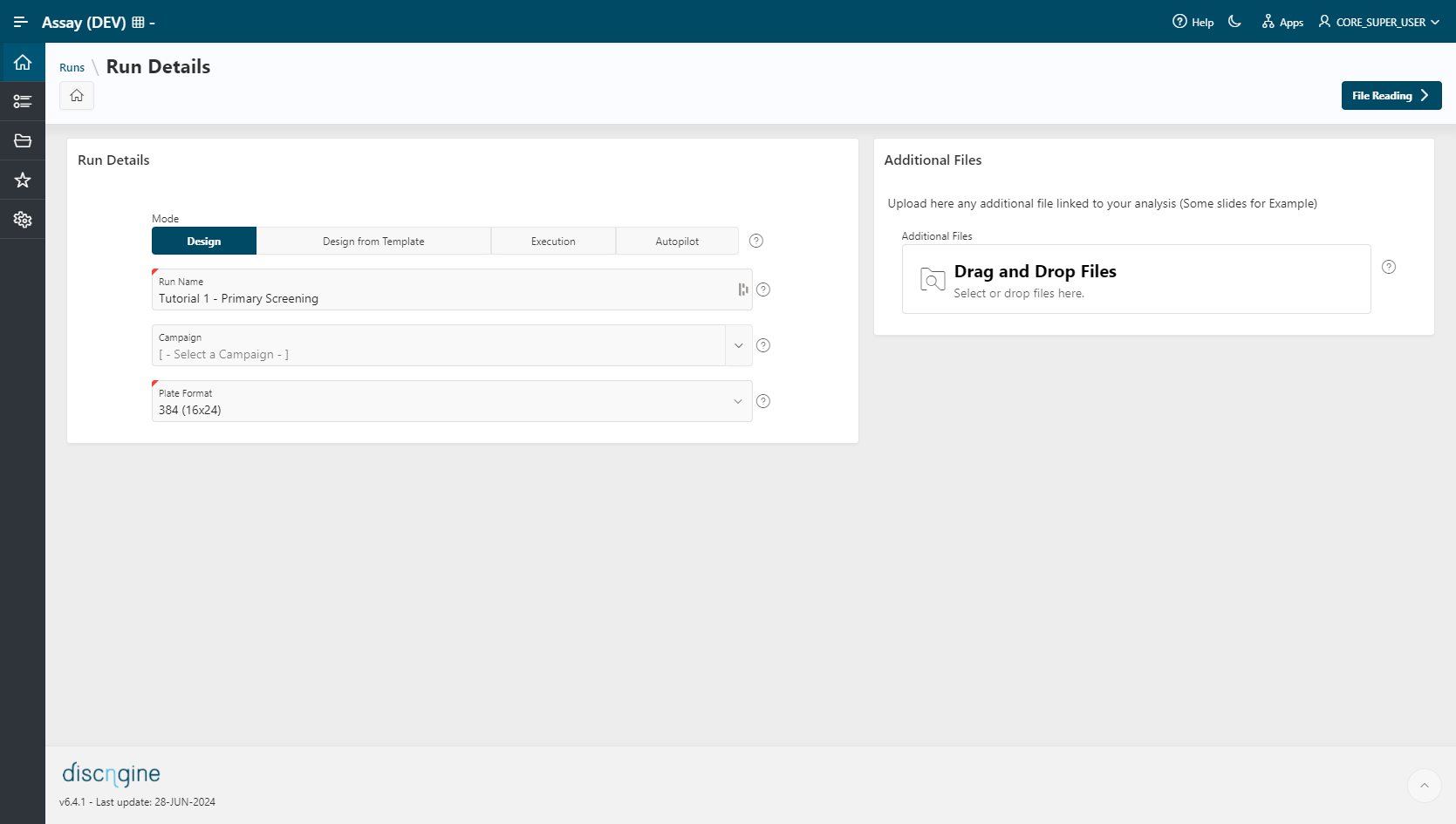
To create a new run, click the New Run button.

Select Mode as Design Mode.
Enter a Run Name.
Specify the plate format to use: 384 (16x24).
Go to the File Reading step.

Run Creation

Info

Run Template is only mandatory in Execution Mode. This option in Design Mode can be used to create a new analysis based on an existing workflow template.

File Reading¶

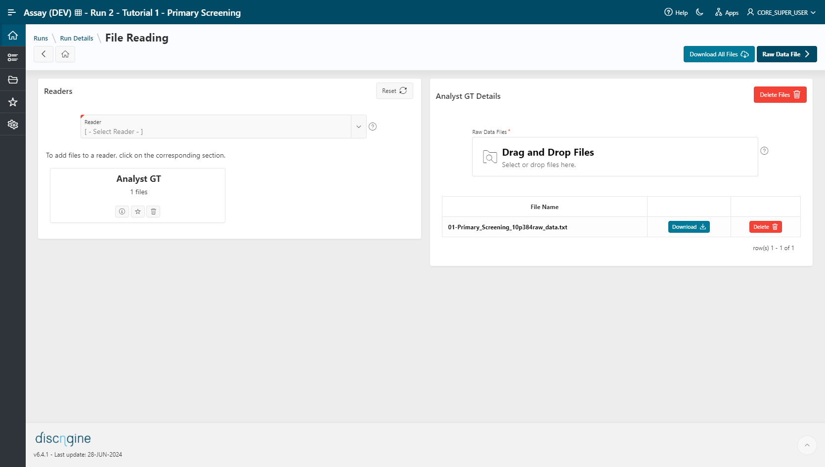
Select Analyst GT (TAB) as a reader.
Select the file 01-Primary_Screening_10p384raw_data in the upload section. The file is automatically uploaded upon selection and listed in the table below.
Go to the Raw Data File step.

File Reading step: Select a Reader and upload file(s)

Raw Data File¶

The Number of Measurements per Plate (1) and the READOUT Alias (READOUT1) are already set.
Go to the Plate Mapping step.

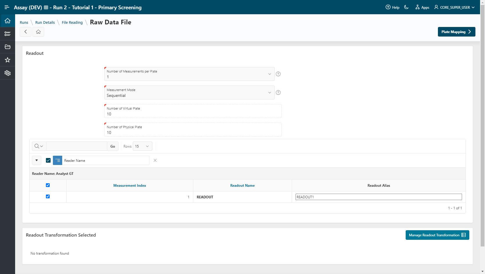
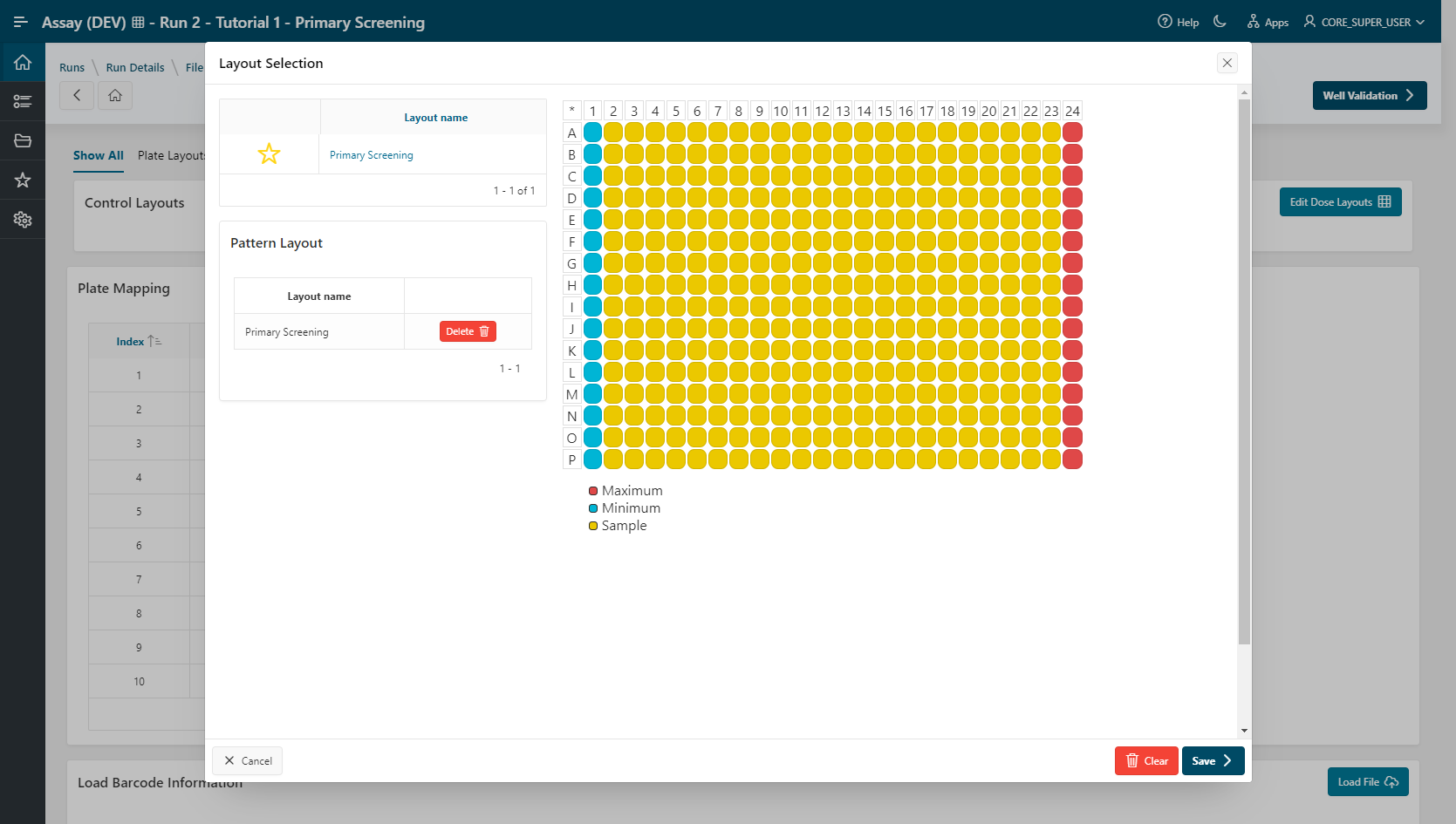
Raw Data File step: Adjust number of measurement and add basic transformations

Plate Mapping¶

Click Edit Control Layouts in the Control Layouts section.
Select the control layout named Primary_Screening (Minimum control in column 1 and maximum control in column 24).
Click the Save button.

Plate Mapping Step: Assign Plate Layout for your analysis

Info

Barcode information is not needed in this tutorial. This section allows users to set plate barcodes using a file with two columns (Plate_Index / Barcode).

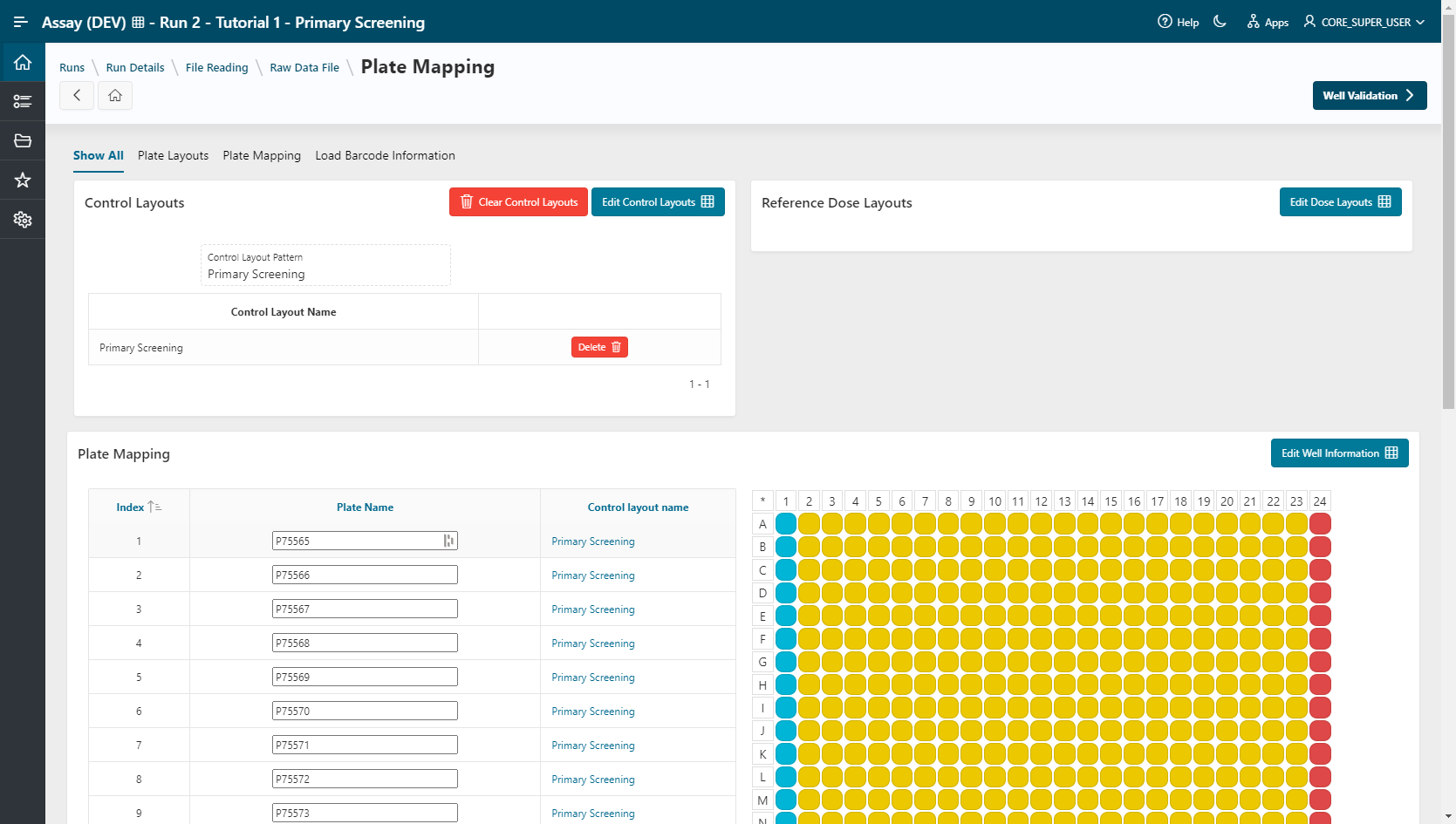
Plate Mapping Step: Assign Plate Layout for your analysis

Go to the Well Validation step.

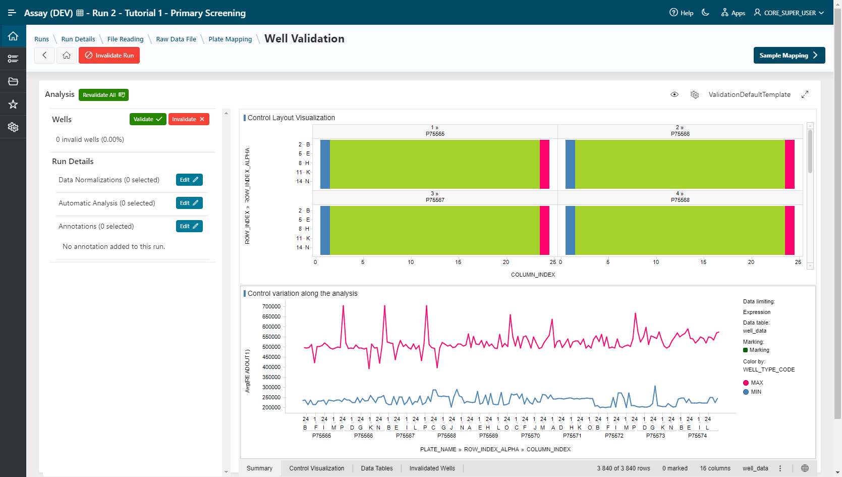
Well Validation¶

Select your visualization tool:

Info

If you are using Spotfire Analyst Client, or if only one visualization tool is installed in your environment, this step will be skipped.

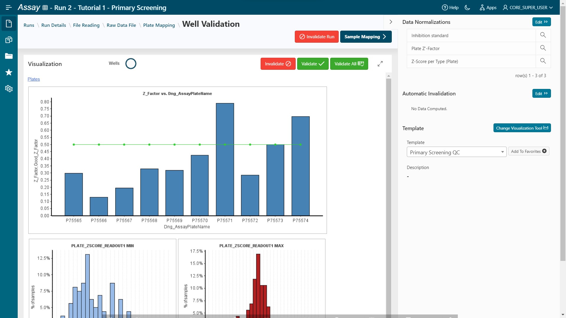
TIBCO Spotfire Webplayer (Template: ValidationDefaultTemplate)

Well Validation step with TIBCO Spotfire tool

Pipeline Pilot (Template: Plate Heat Maps)

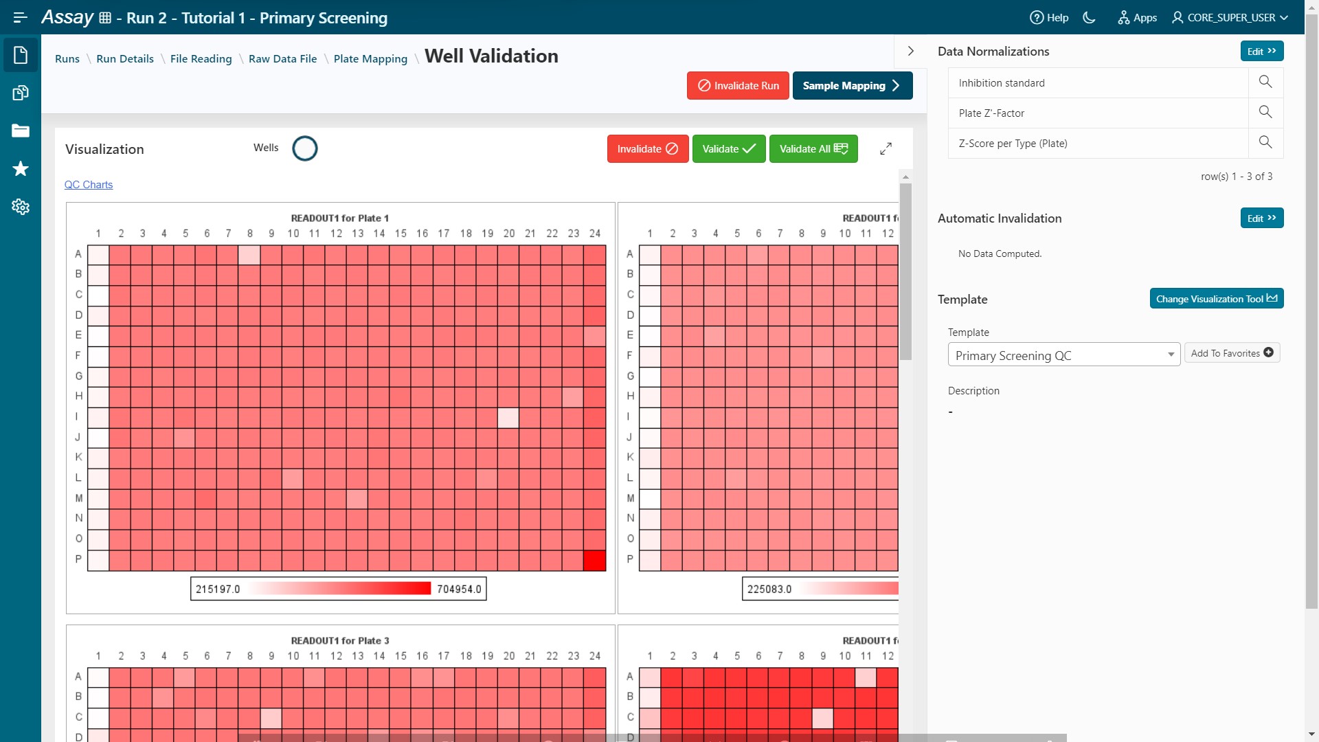
Well Validation step with BIOVIA Pipeline Pilot tool

Results are loaded.

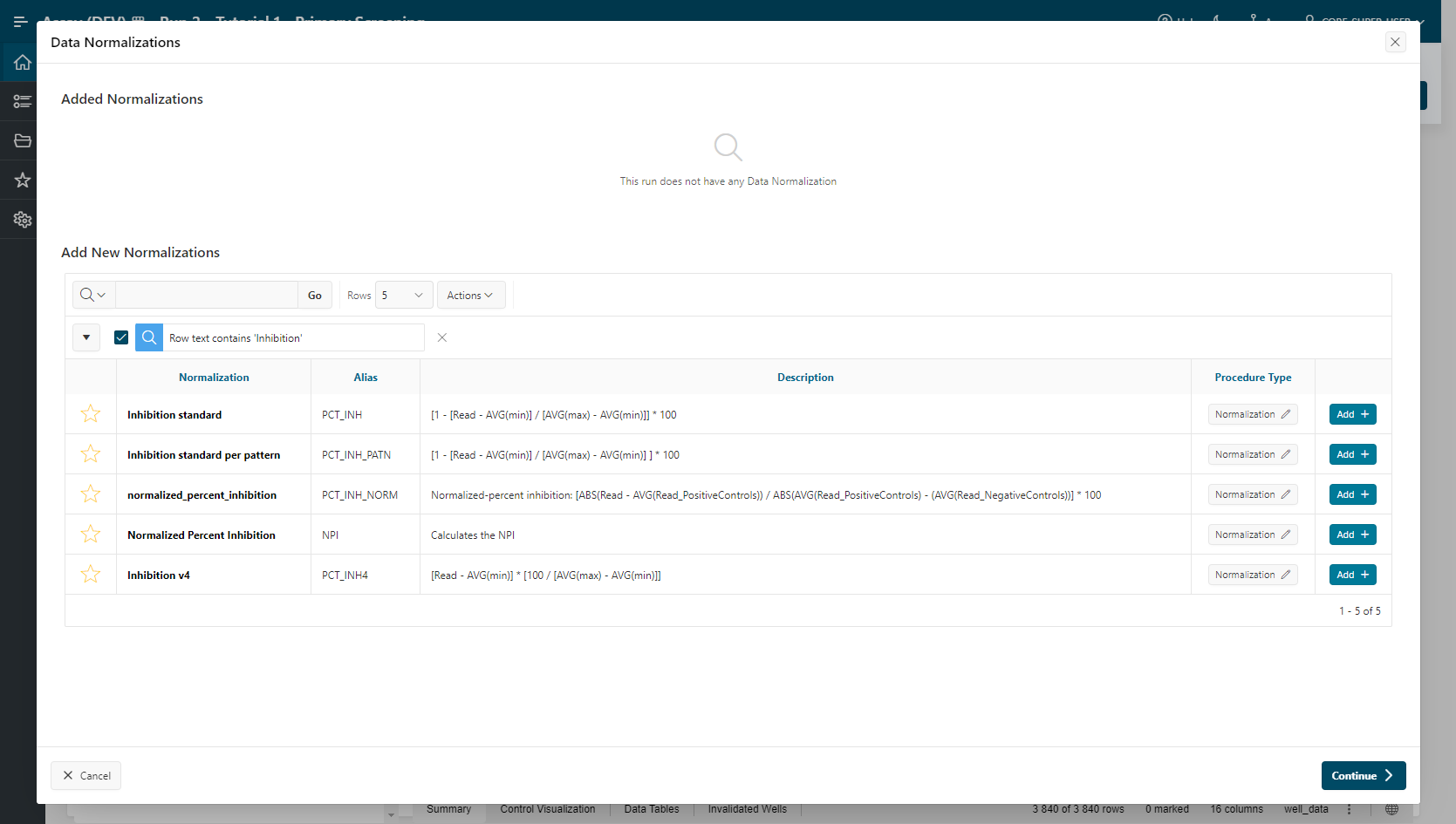
Add Data Normalizations:

In the left panel, next to the "Data Normalization" summary, click Edit to open the Data Normalizations modal.
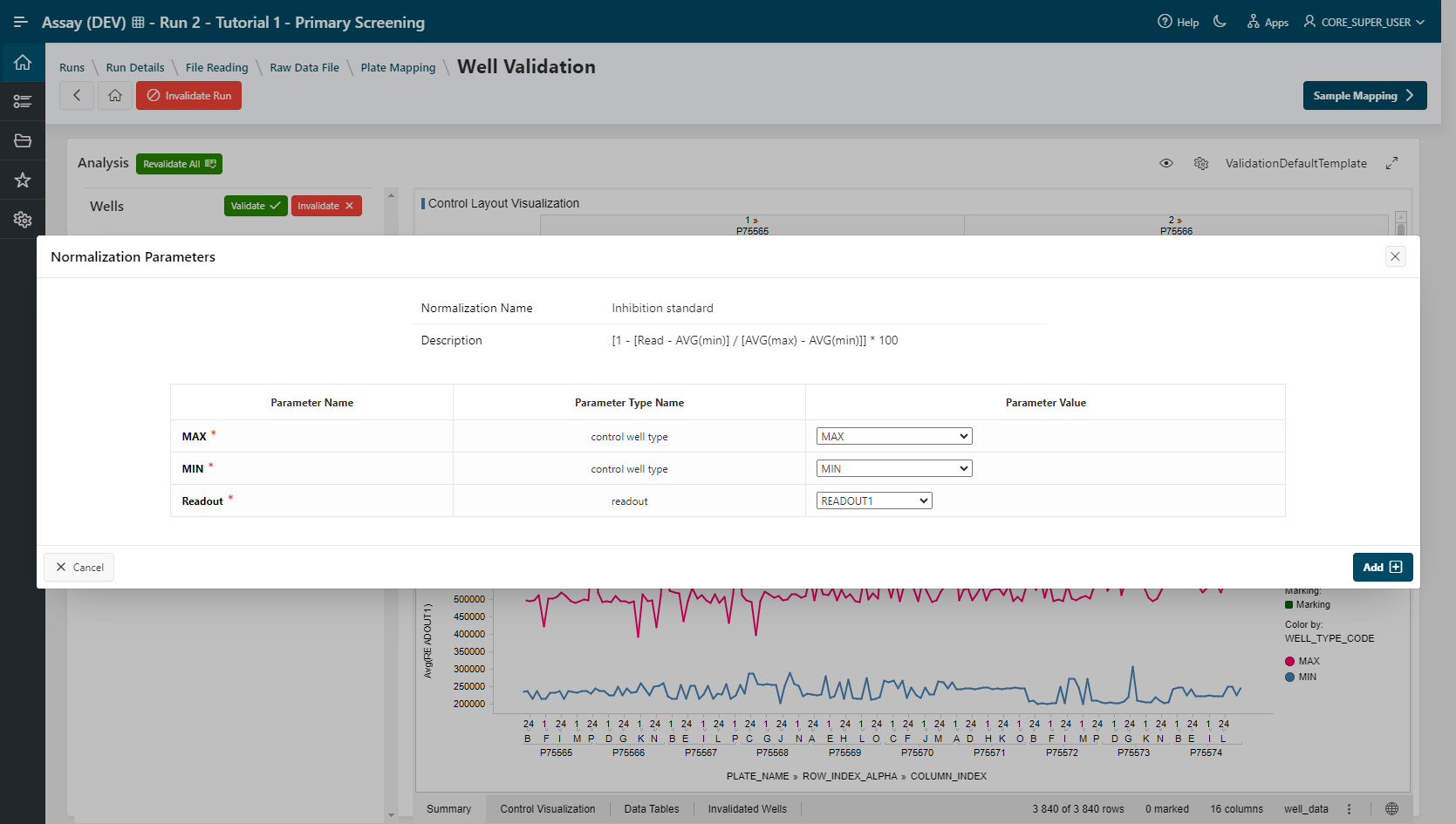
Look for the "Inhibition Standard" procedure and click on Add:
- Value READOUT1, MIN, MAX are selected.
- Click Add.

Well Validation step: Add normalization(s)

The Inhibition Standard normalization is listed in the Data Normalization Summary section.

Repeat the same action for Plate Z'-factor normalization:
- Values READOUT1, MIN and MAX are selected.
- Click Add.

The Plate Z-factor normalization is listed in the Data Normalization Summary section.

Do the same for Z-Score per Type (Plate) normalization:
- Value READOUT1 is selected.
- Click Add.

The Z-Score per Type (Plate) normalization is listed in the Data Normalization Summary section.

Summary of Normalization added

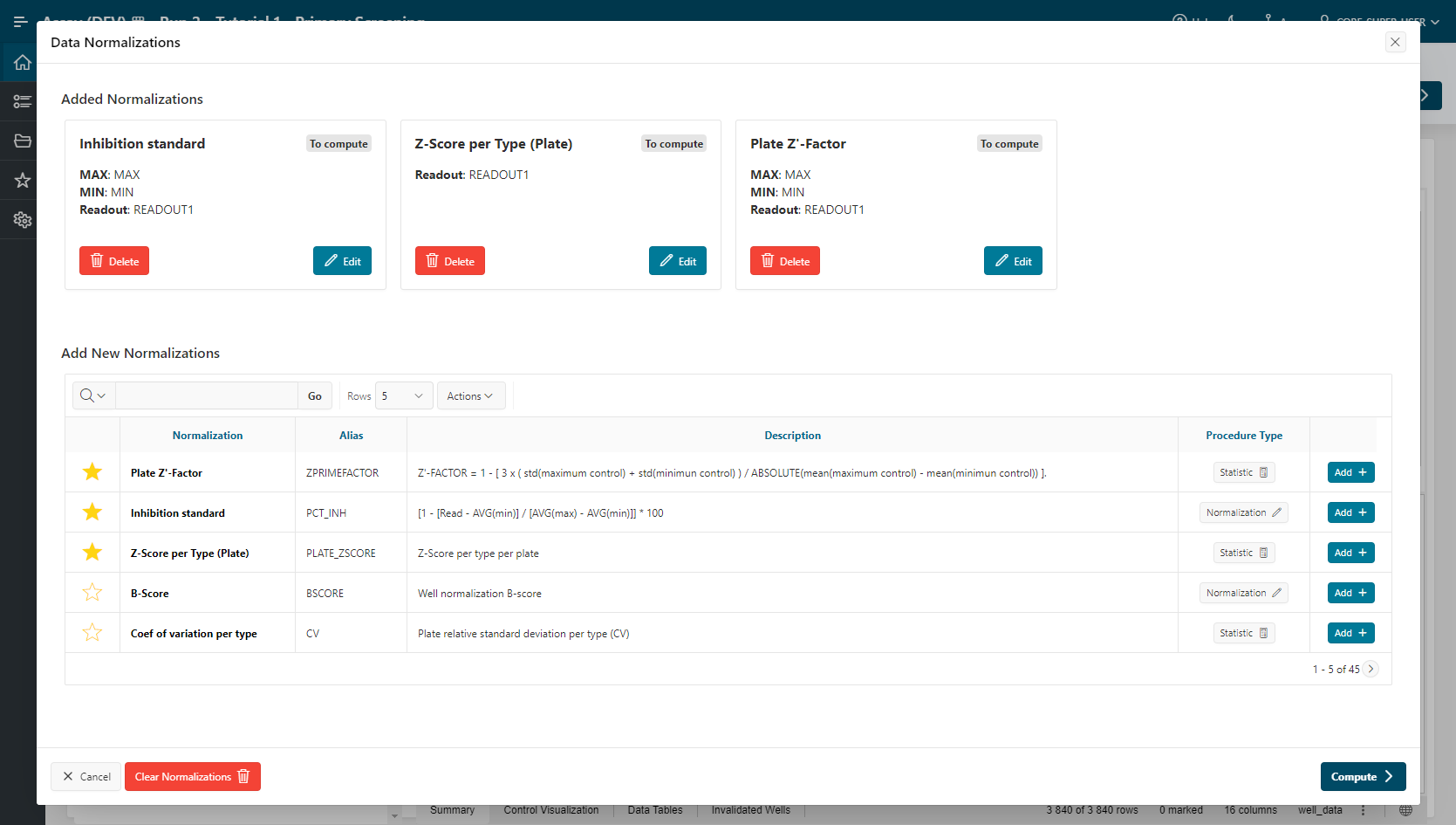
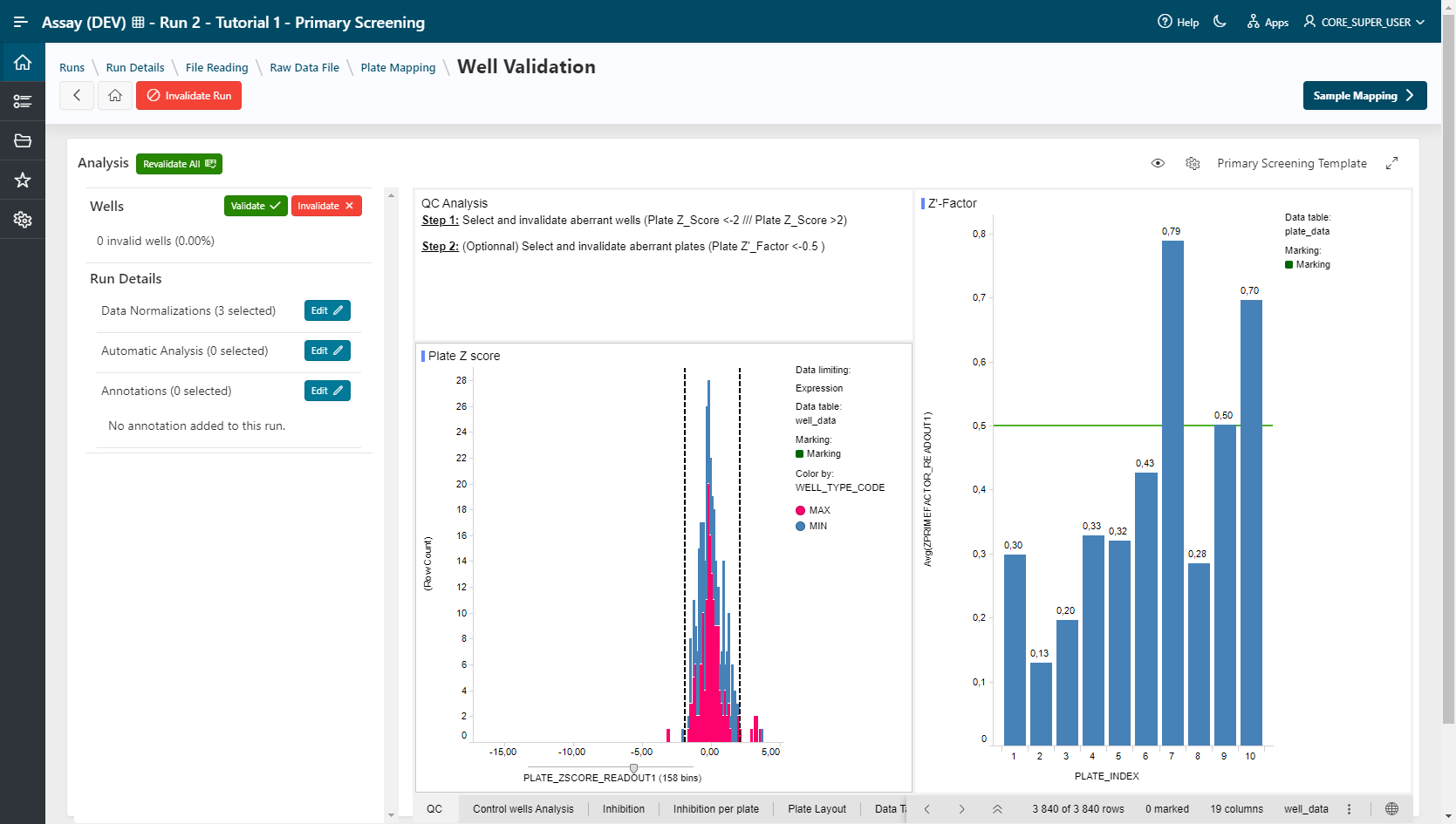
Click Compute.

All normalizations are processed. Select another visualization template by clicking on the gears button above the current visualization.

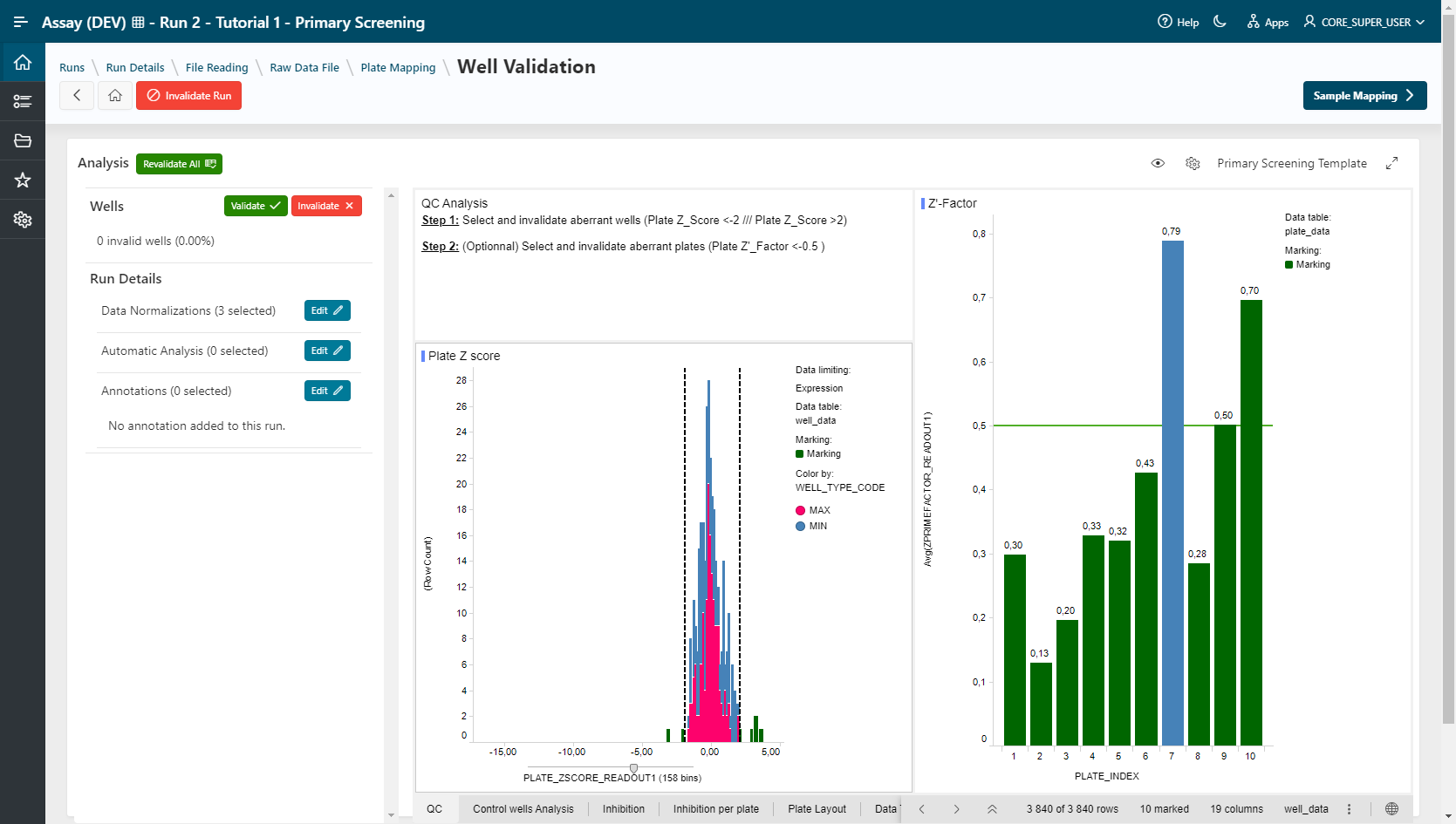
Well Validation step: Change visualization

Primary_Screening_Template for TIBCO Spotfire WebPlayer.

Well Validation step: Apply Primary_Screening_Template visualization Template

Primary Screening QC for Pipeline Pilot.

Well Validation step: Apply Primary Screening QC Template visualization Template

You can also create a new one and save it (see developer guide to register a new Pipeline Pilot Protocol in Assay).

For QC Validation, select aberrant wells in the visualization and click on the Well Validation step: Invalidation button button. Multiple selection is allowed by holding the Ctrl key.

After each invalidation, the normalizations will be relaunched in order to recalculate based on your selection.

Example

Plate_ZSCORE_READOUT1 < -2 or Plate_ZSCORE_READOUT1 > 2. (10 wells are invalidated) and all normalizations are recomputed.

Well Validation step: Invalidate wells based on Plate Z-Score

Go to the Sample Mapping step.

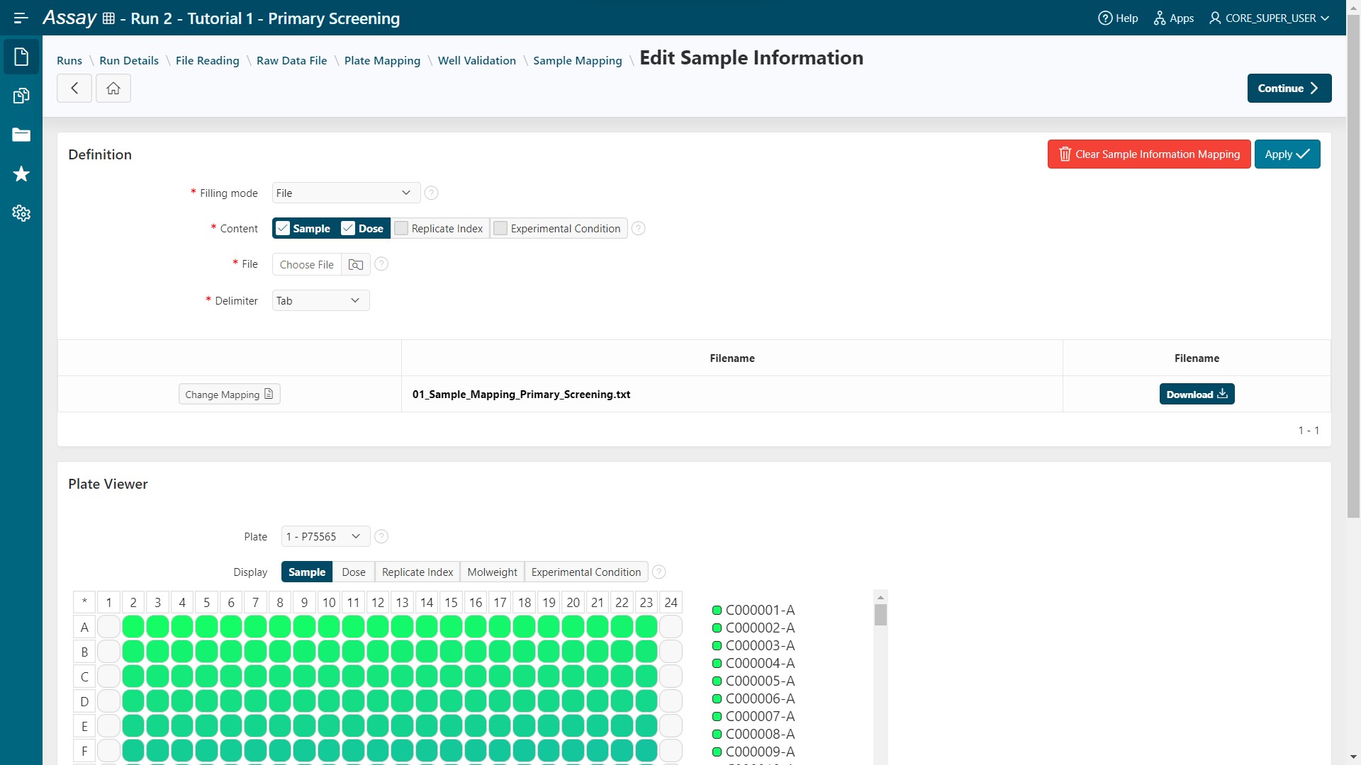
Sample Mapping¶

Select filling mode File and tick Sample and Dose for content.
Load the file 01_Sample_Mapping_Primary_Screening.
Click on the Apply button.

Samples and doses are filled in.

Sample Mapping step: Mapped from file

Click on the Continue button. Samples and doses are mapped for all plates.

Sample Mapping step: Sample and doses are mapped for all plates

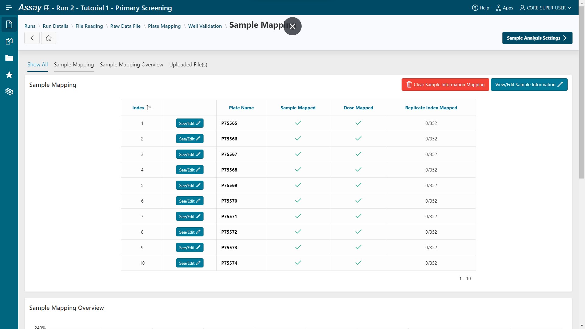
Click on the Sample Analysis Settings button.

Sample Analysis Setting¶

Select SampleName as Parameters to Aggregate.
Select the Series: PCT_INH_READOUT1.

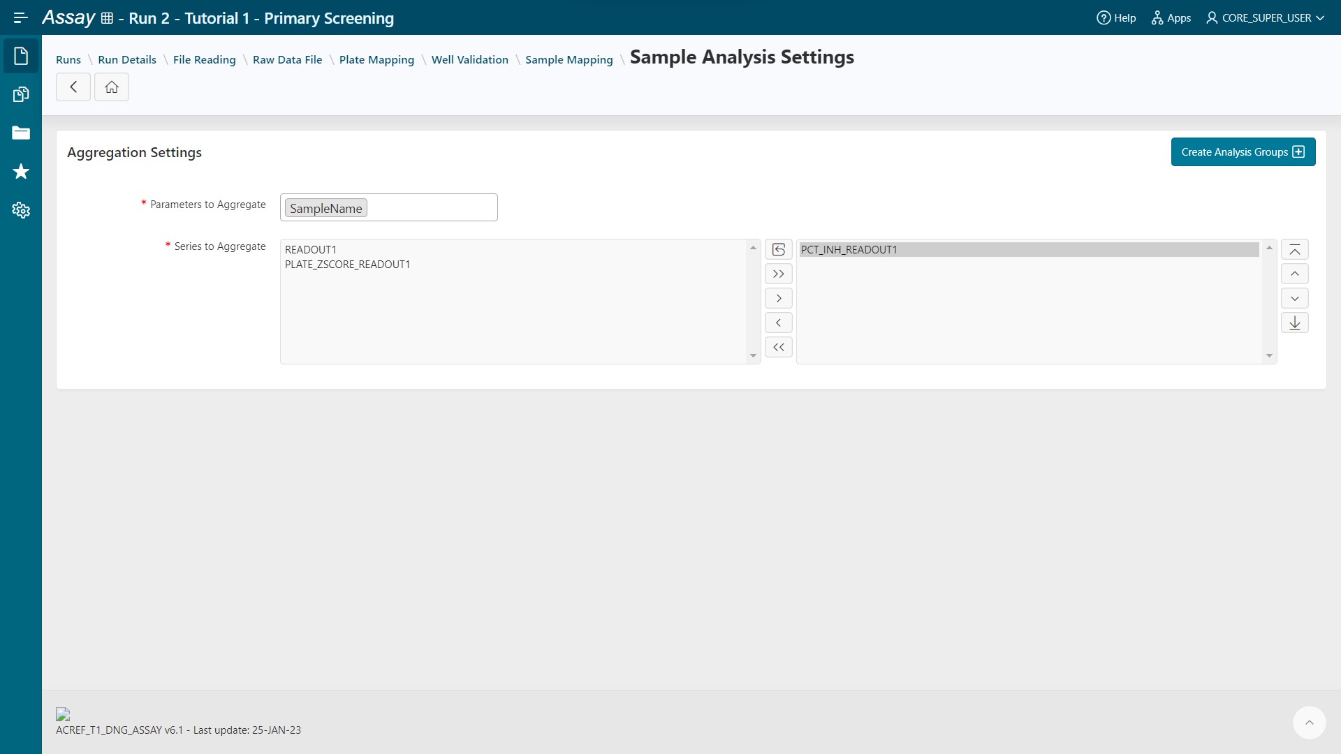
Sample Analysis Settings step: Set aggregation parameters

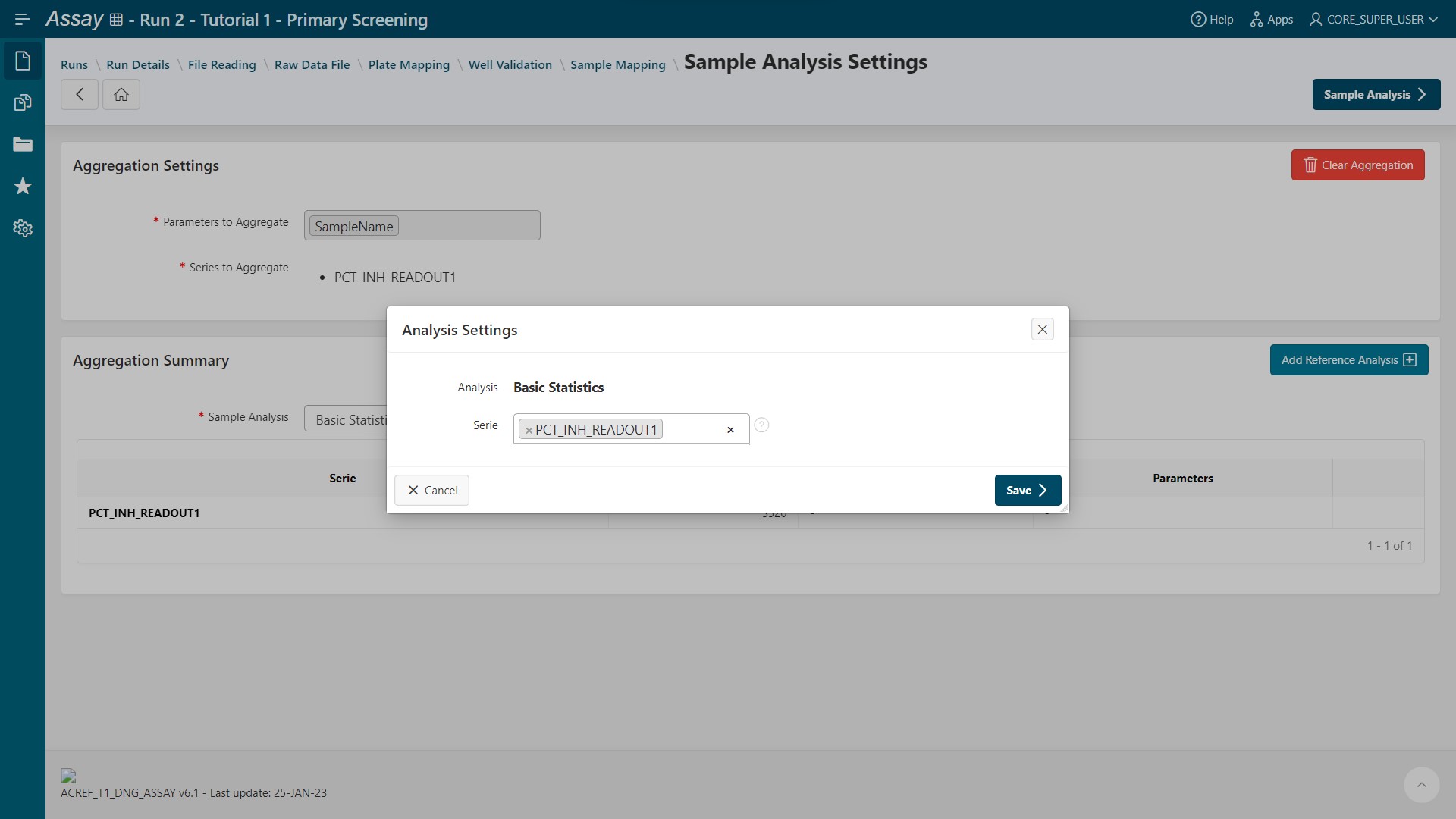
Click on the Create Analysis Groups button: 3520 groups are created.
Select the Analysis Basic Statistics then click on the Add Reference Analysis button.

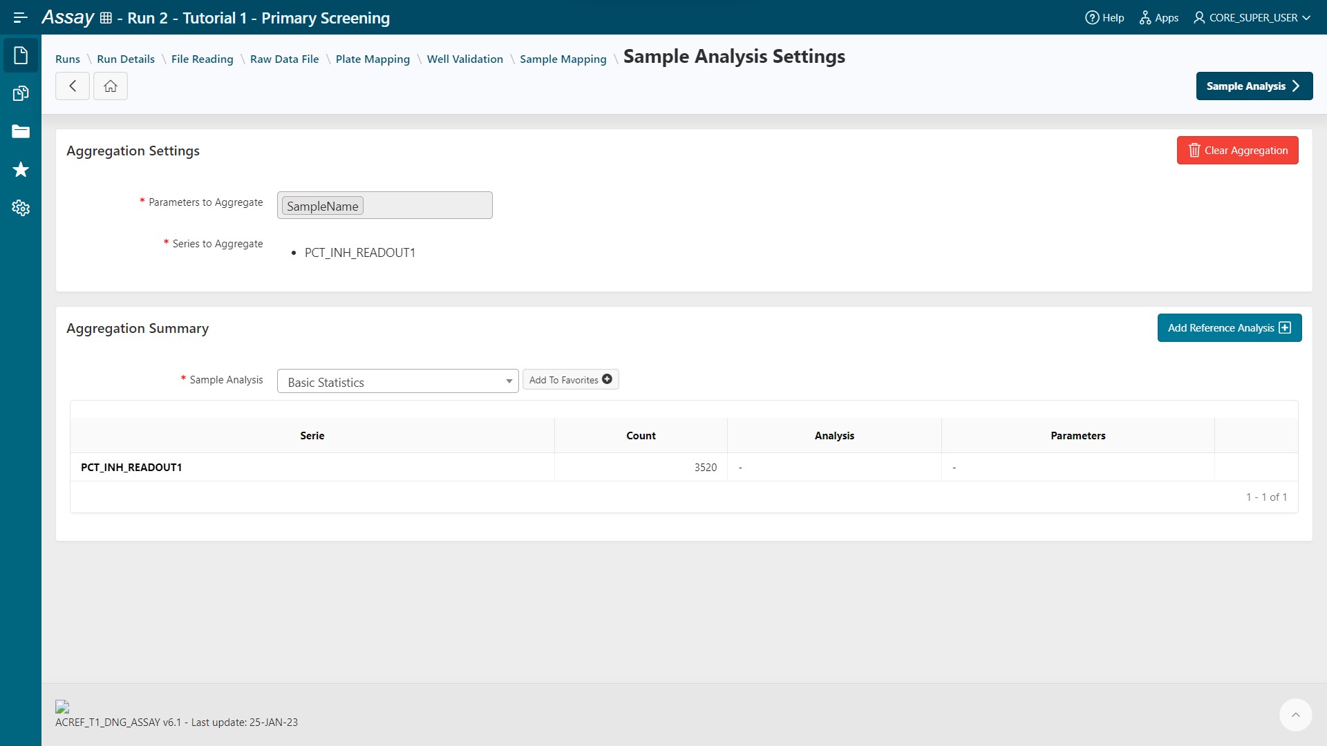
Sample Analysis Setting step: Aggregation Analysis

Click on the Save button to apply basic statistics to all series.

Sample Analysis Settings step: Analysis parameters.

Go to the Sample Analysis step.

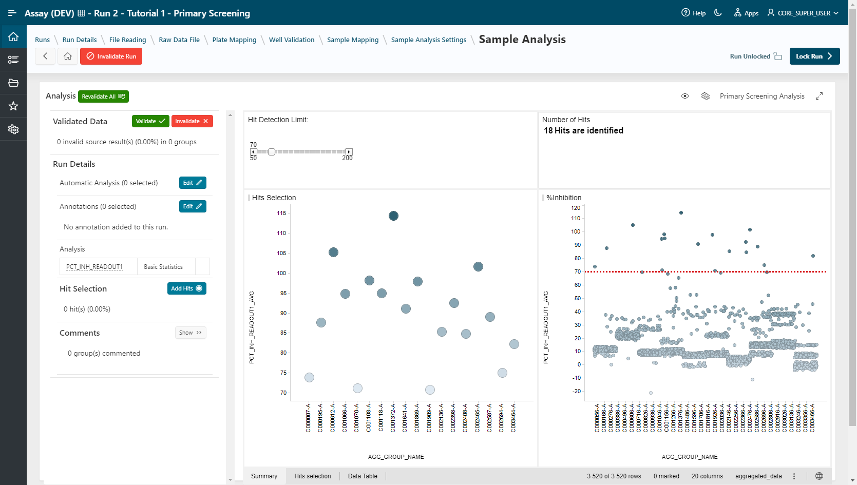
Sample Analysis¶

Select your Visualization Tool:

TIBCO Spotfire Webplayer
Pipeline Pilot

Info

This step is only available if 2 visualization tools are installed. Otherwise, this step will be skipped.

Apply an existing template (Spotfire) or protocol (Pipeline Pilot):

Primary_Screening_Analysis for TIBCO Spotfire Webplayer

Sample Analysis Results using TIBCO Spotfire with the right panel closed

Tip

The space occupied by the visualization can be optimized to your liking by clicking on the full screen icon icon and the icon

Source and Final Results Table Sample for Pipeline Pilot

Sample Analysis Results using Pipeline Pilot

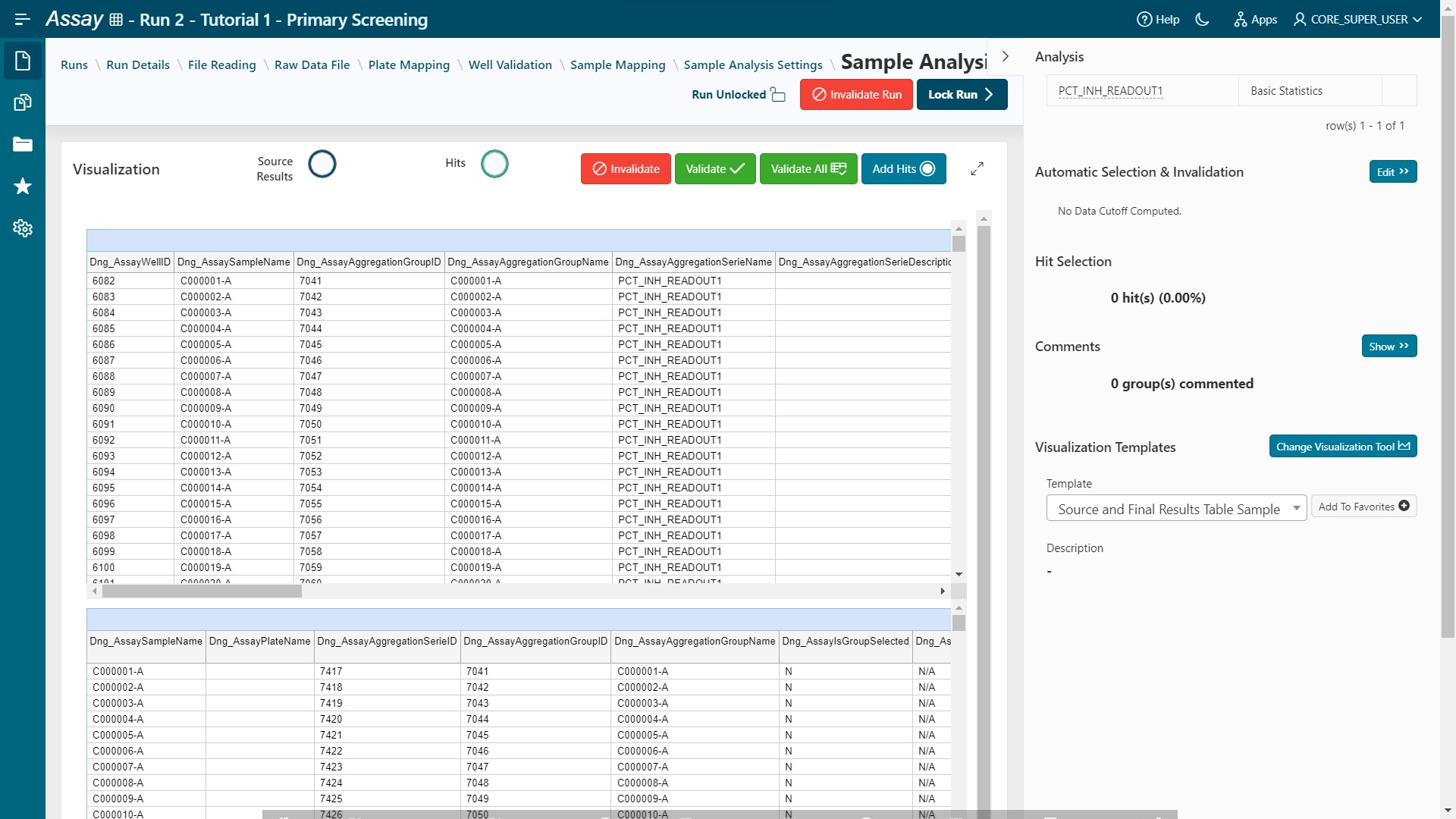
For Hit Selection, select points (hits) in the visualization and add them to a list by clicking on the Add Hits button. This selection can be exported in CSV format (export button) or used to create a list that can be used in the Sample application.

Lock your Analysis using the Lock Run button.
Go to Publisher step.

Publisher Selection & Workflow Template Creation¶

Select a target publisher (depending on what is installed – None, Warehouse or BIOVIA Project Data). For more information on publishing data see the Publisher guide.

Selection of a publisher.

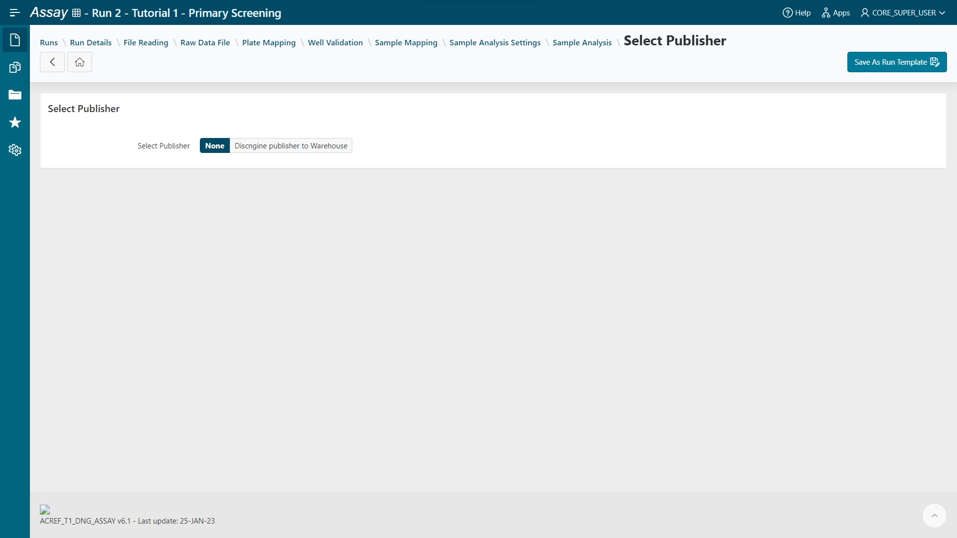
Save your analysis by clicking on Save As Run Template. The template will be used later in the execution mode.

Save a Run Template.

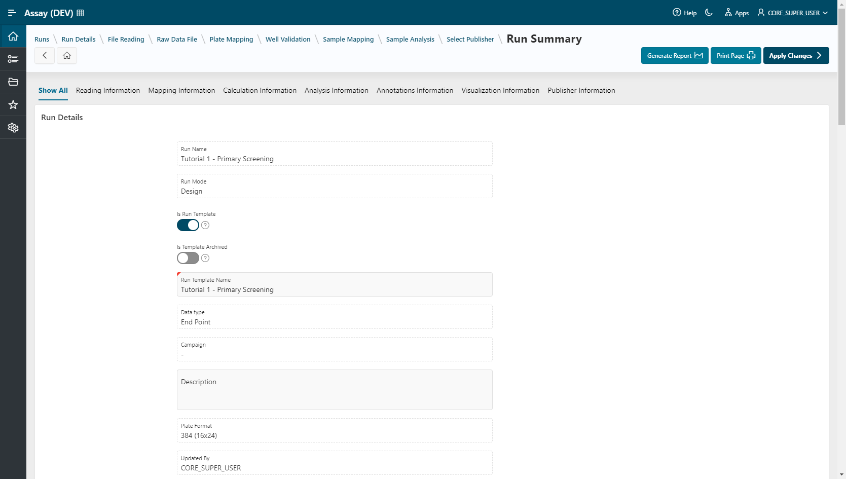
Give a name and description to the run template.
Click on Apply Changes to save your modifications.

Info

Once the run template is saved, the screeners can use it in Execution Mode, following this tutorial